Static maps

Over the course of the last weeks, we have already become familiar to plotting basic static maps using geopandas.GeoDataFrame.plot(), for instance in lessons 2, 3, and 4. We also learnt that geopandas.GeoDataFrame.plot() uses the matplotlib.pyplot library, and that most of its arguments and options are accepted by geopandas.

To refresh our memory about the basics of plotting maps, let’s create a static accessibility map of the Helsinki metropolitan area, that also shows roads and metro lines (three layers, overlayed onto each other). Remember that the input data sets need to be in the same coordinate system!

Data

We will use three different data sets:

• the travel time to the Helsinki railway station we used in lesson 4, which is in DATA_DIRECTORY / "helsinki_region_travel_times_to_railway_station",

• the Helsinki Metro network, available via WFS from the city’s map services, and

• a simplified network of the most important roads in the metropolitan region, also available via WFS from the same endpoint.

import pathlib
NOTEBOOK_PATH = pathlib.Path().resolve()
DATA_DIRECTORY = NOTEBOOK_PATH / "data"

import geopandas
import numpy

accessibility_grid = geopandas.read_file(
    DATA_DIRECTORY
    / "helsinki_region_travel_times_to_railway_station"
    / "helsinki_region_travel_times_to_railway_station.gpkg"
)
accessibility_grid["pt_r_t"] = accessibility_grid["pt_r_t"].replace(-1, numpy.nan)

WFS_BASE_URL = (
    "https://kartta.hel.fi/ws/geoserver/avoindata/wfs"
    "?service=wfs"
    "&version=2.0.0"
    "&request=GetFeature"
    "&srsName=EPSG:3879"
    "&typeName={layer:s}"
)

metro = (
    geopandas.read_file(
        WFS_BASE_URL.format(layer="avoindata:Seutukartta_liikenne_metro_rata")
    )
    .set_crs("EPSG:3879")
)
roads = (
    geopandas.read_file(
        WFS_BASE_URL.format(layer="avoindata:Seutukartta_liikenne_paatiet")
    )
    .set_crs("EPSG:3879")
)

Coordinate reference systems

Remember that different geo-data frames need to be in same coordinate system before plotting them in the same map. geopandas.GeoDataFrame.plot() does not reproject data automatically.

You can always check it with a simple assert statement.

assert accessibility_grid.crs == metro.crs == roads.crs, "Input data sets’ CRS differs"

---------------------------------------------------------------------------
AssertionError                            Traceback (most recent call last)
Cell In [3], line 1
----> 1 assert accessibility_grid.crs == metro.crs == roads.crs, "Input data sets’ CRS differs"

AssertionError: Input data sets’ CRS differs

If multiple data sets do not share a common CRS, first, figure out which CRS they have assigned (if any!), then transform the data into a common reference system:

accessibility_grid.crs

<Derived Projected CRS: EPSG:3067>
Name: ETRS89 / TM35FIN(E,N)
Axis Info [cartesian]:
- E[east]: Easting (metre)
- N[north]: Northing (metre)
Area of Use:
- name: Finland - onshore and offshore.
- bounds: (19.08, 58.84, 31.59, 70.09)
Coordinate Operation:
- name: TM35FIN
- method: Transverse Mercator
Datum: European Terrestrial Reference System 1989 ensemble
- Ellipsoid: GRS 1980
- Prime Meridian: Greenwich

metro.crs

<Derived Projected CRS: EPSG:3879>
Name: ETRS89 / GK25FIN
Axis Info [cartesian]:
- N[north]: Northing (metre)
- E[east]: Easting (metre)
Area of Use:
- name: Finland - nominally onshore between 24°30'E and 25°30'E but may be used in adjacent areas if a municipality chooses to use one zone over its whole extent.
- bounds: (24.5, 59.94, 25.5, 68.9)
Coordinate Operation:
- name: Finland Gauss-Kruger zone 25
- method: Transverse Mercator
Datum: European Terrestrial Reference System 1989 ensemble
- Ellipsoid: GRS 1980
- Prime Meridian: Greenwich

roads.crs

<Derived Projected CRS: EPSG:3879>
Name: ETRS89 / GK25FIN
Axis Info [cartesian]:
- N[north]: Northing (metre)
- E[east]: Easting (metre)
Area of Use:
- name: Finland - nominally onshore between 24°30'E and 25°30'E but may be used in adjacent areas if a municipality chooses to use one zone over its whole extent.
- bounds: (24.5, 59.94, 25.5, 68.9)
Coordinate Operation:
- name: Finland Gauss-Kruger zone 25
- method: Transverse Mercator
Datum: European Terrestrial Reference System 1989 ensemble
- Ellipsoid: GRS 1980
- Prime Meridian: Greenwich

roads = roads.to_crs(accessibility_grid.crs)
metro = metro.to_crs(accessibility_grid.crs)

assert accessibility_grid.crs == metro.crs == roads.crs, "Input data sets’ CRS differs"

Plotting a multi-layer map

Check your understanding

Complete the next steps at your own pace (clear out the code cells first). Make sure to revisit previous lessons if you feel unsure how to complete a task.

• Visualise a multi-layer map using the geopandas.GeoDataFrame.plot() method;

• first, plot the accessibility grid using a ‘quantiles’ classification scheme,

• then, add roads network and metro lines in the same plot (remember the ax parameter)

Remember the following options that can be passed to plot():

• style the polygon layer:

  • define a classification scheme using the scheme parameter

  • change the colour map using cmap

  • control the layer’s transparency the alpha parameter (0 is fully transparent, 1 fully opaque)

• style the line layers:

  • adjust the line colour using the color parameter

  • change the linewidth, as needed

The layers have different extents (roads covers a much larger area). You can use the axes’ (ax) methods set_xlim() and set_ylim() to set the horizontal and vertical extents of the map (e.g., to a geo-data frame’s total_bounds).

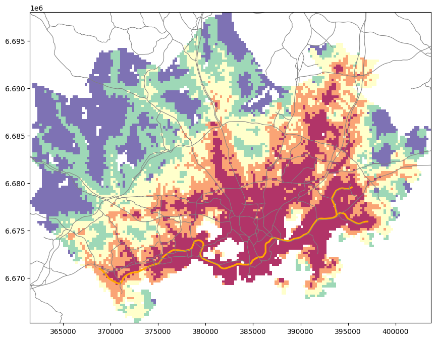
ax = accessibility_grid.plot(
    figsize=(12, 8),

    column="pt_r_t",
    scheme="quantiles",
    cmap="Spectral",
    linewidth=0,
    alpha=0.8
)

metro.plot(
    ax=ax,
    color="orange",
    linewidth=2.5
)

roads.plot(
    ax=ax,
    color="grey",
    linewidth=0.8
)

minx, miny, maxx, maxy = accessibility_grid.total_bounds
ax.set_xlim(minx, maxx)
ax.set_ylim(miny, maxy)

(6665250.00004393, 6698000.000038021)

Adding a legend

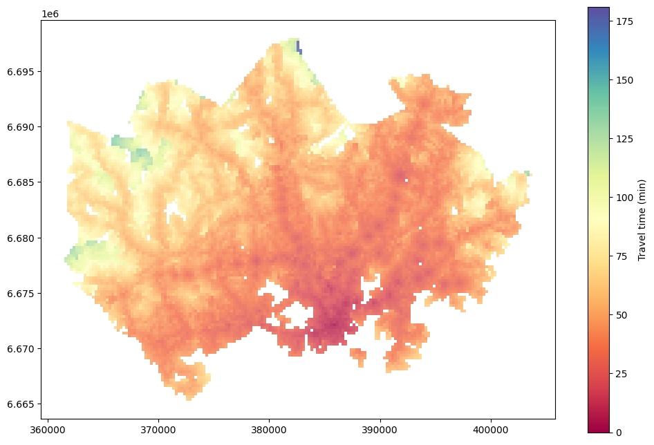
To plot a legend for a map, add the legend=True parameter.

For figures without a classification scheme, the legend consists of a colour gradient bar. The legend is an instance of matplotlib.pyplot.colorbar.Colorbar, and all arguments defined in legend_kwds are passed through to it. See below how to use the label property to set the legend title:

ax = accessibility_grid.plot(
    figsize=(12, 8),

    column="pt_r_t",
    cmap="Spectral",
    linewidth=0,
    alpha=0.8,

    legend=True,
    legend_kwds={"label": "Travel time (min)"}
)

Set other Colorbar parameters

Check out matplotlib.pyplot.colorbar.Colorbar’s documentation and experiment with other parameters! Anything you add to the legend_kwds dictionary will be passed to the colour bar.

---

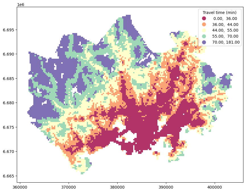
For figures that use a classification scheme, on the other hand, plot() creates a matplotlib.legend.Legend. Again, legend_kwds are passed through, but the parameters are slightly different: for instance, use title instead of label to set the legend title:

accessibility_grid.plot(
    figsize=(12, 8),

    column="pt_r_t",
    scheme="quantiles",
    cmap="Spectral",
    linewidth=0,
    alpha=0.8,

    legend=True,
    legend_kwds={"title": "Travel time (min)"}
)

<AxesSubplot: >

Set other Legend parameters

Check out matplotlib.pyplot.legend.Legend’s documentation, and experiment with other parameters! Anything you add to the legend_kwds dictionary will be passed to the legend.

What legend_kwds keyword would spread the legend onto two columns?

Adding a base map

For better orientation, it is often helpful to add a base map to a map plot. A base map, for instance, from map providers such as OpenStreetMap or Stamen, adds streets, place names, and other contextual information.

The Python package contextily takes care of downloading the necessary map tiles and rendering them in a geopandas plot.

Web Mercator

Map tiles from online map providers are typically in Web Mercator projection (EPSG:3857. It is generally advisable to transform all other layers to EPSG:3857, too.

accessibility_grid = accessibility_grid.to_crs("EPSG:3857")
metro = metro.to_crs("EPSG:3857")
roads = roads.to_crs("EPSG:3857")

To add a base map to an existing plot, use the contextily.add_basemap() function, and supply the plot’s ax object obtained in an earlier step.

import contextily

ax = accessibility_grid.plot(
    figsize=(12, 8),

    column="pt_r_t",
    scheme="quantiles",
    cmap="Spectral",
    linewidth=0,
    alpha=0.8,

    legend=True,
    legend_kwds={"title": "Travel time (min)"}
)
contextily.add_basemap(ax)

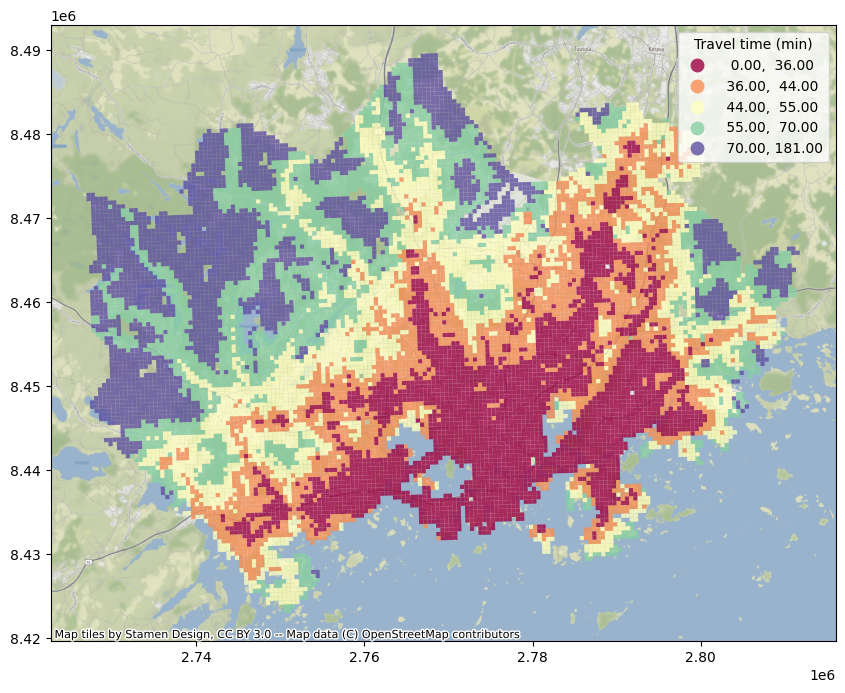
By default, contextily uses the Stamen Terrain as a base map, but there are many other online maps to choose from. Any of the other contextily.providers (see link above) can be passed as a source to add_basemap(). For instance, use OpenStreetMap in its default Mapnik style:

ax = accessibility_grid.plot(
    figsize=(12, 8),

    column="pt_r_t",
    scheme="quantiles",
    cmap="Spectral",
    linewidth=0,
    alpha=0.8,

    legend=True,
    legend_kwds={"title": "Travel time (min)"}
)
contextily.add_basemap(
    ax,
    source=contextily.providers.OpenStreetMap.Mapnik
)

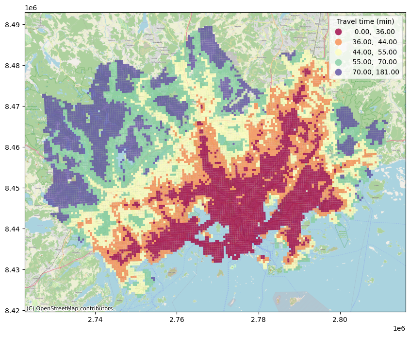
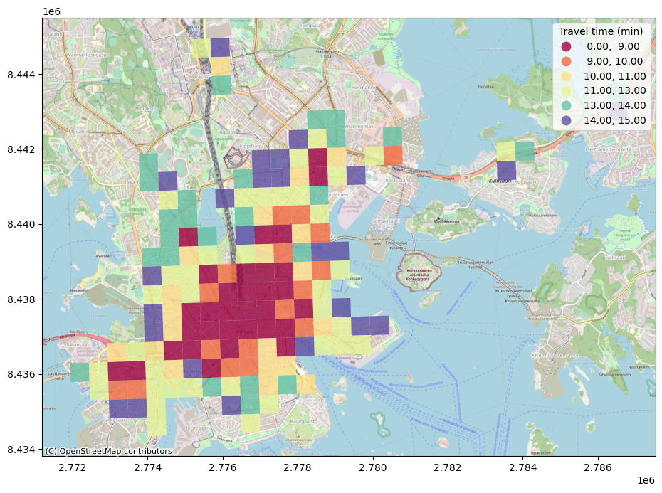
In this zoom level, the benefits from using OpenStreetMap (such as place names) do not live to their full potential. Let’s look at a subset of the travel time matrix: grid cells that are within 15 minutes from the railway station.

ax = accessibility_grid[accessibility_grid.pt_r_t <= 15].plot(
    figsize=(12, 8),

    column="pt_r_t",
    scheme="quantiles",
    k=7,
    cmap="Spectral",
    linewidth=0,
    alpha=0.8,

    legend=True,
    legend_kwds={"title": "Travel time (min)"}
)
contextily.add_basemap(
    ax,
    source=contextily.providers.OpenStreetMap.Mapnik
)

/home/docs/checkouts/readthedocs.org/user_builds/autogis-site/envs/2022/lib/python3.10/site-packages/mapclassify/classifiers.py:238: UserWarning: Warning: Not enough unique values in array to form k classes
  Warn(
/home/docs/checkouts/readthedocs.org/user_builds/autogis-site/envs/2022/lib/python3.10/site-packages/mapclassify/classifiers.py:241: UserWarning: Warning: setting k to 6
  Warn("Warning: setting k to %d" % k_q, UserWarning)

Finally, we can modify the attribution (copyright notice) displayed in the bottom left of the map plot. Note that you should always respect the map providers’ terms of use, which typically include a data source attribution (contextily’s defaults take care of this). We can and should, however, add a data source for any layer we added, such as the travel time matrix data set:

ax = accessibility_grid[accessibility_grid.pt_r_t <= 15].plot(
    figsize=(12, 8),

    column="pt_r_t",
    scheme="quantiles",
    k=7,
    cmap="Spectral",
    linewidth=0,
    alpha=0.8,

    legend=True,
    legend_kwds={"title": "Travel time (min)"}
)
contextily.add_basemap(
    ax,
    source=contextily.providers.OpenStreetMap.Mapnik,
    attribution=(
        "Travel time data (c) Digital Geography Lab, "
        "map data (c) OpenStreetMap contributors"
    )
)

/home/docs/checkouts/readthedocs.org/user_builds/autogis-site/envs/2022/lib/python3.10/site-packages/mapclassify/classifiers.py:238: UserWarning: Warning: Not enough unique values in array to form k classes
  Warn(
/home/docs/checkouts/readthedocs.org/user_builds/autogis-site/envs/2022/lib/python3.10/site-packages/mapclassify/classifiers.py:241: UserWarning: Warning: setting k to 6
  Warn("Warning: setting k to %d" % k_q, UserWarning)