Static maps#

Data#

You should have following Shapefiles in the data folder:

addresses.shp
metro.shp
roads.shp
some.geojson
TravelTimes_to_5975375_RailwayStation.shp

In case you don’t see the required files in the data folder, you can download them from this link.

You can download and extract the data into a folder data using these commands:

    cd autogis/notebooks/L5
    wget https://github.com/Automating-GIS-processes/Lesson-5-Making-Maps/raw/master/data/dataE5.zip
    unzip dataE5.zip -d data

Static maps in geopandas#

We have already plotted basic static maps using geopandas during the previous weeks of this course. Remember that when using the plot() method in geopandas, we are actually using the tools available from matplotlib pyplot.

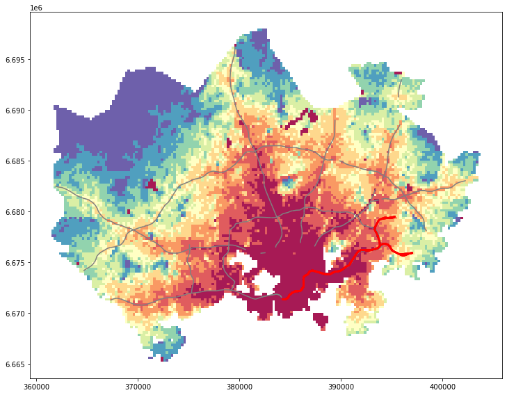
Let’s refresh our memory about the basics of plotting maps by creating a static accessibility map with roads and metro line on it (three layers on top of each other in the same figure). Before plotting the layers, we need to check that they are in the same coordinate reference system.

As usual, we start by importing the useful modules and reading in the input files:

import geopandas as gpd
from pyproj import CRS
import matplotlib.pyplot as plt

# Filepaths
grid_fp = "data/TravelTimes_to_5975375_RailwayStation.shp"
roads_fp = "data/roads.shp"
metro_fp = "data/metro.shp"

# Read files
grid = gpd.read_file(grid_fp)
roads = gpd.read_file(roads_fp)
metro = gpd.read_file(metro_fp)

Let’s check the coordinate reference systems (crs) of the input files.

# Check the crs of each layer
print(roads.crs)
print(metro.crs)
print(grid.crs)

epsg:2392
epsg:2392
epsg:3067

Roads and the metro are in an old Finnish crs (EPSG:2392), while the grid is in ETRS89 / TM35FIN (EPSG:3067):

# Check CRS names
print(f"Roads crs: {CRS(roads.crs).name}")
print(f"Metro crs: {CRS(metro.crs).name}")
print(f"Grid crs: {CRS(grid.crs).name}")

Roads crs: KKJ / Finland zone 2
Metro crs: KKJ / Finland zone 2
Grid crs: ETRS89 / TM35FIN(E,N)

Let’s re-project geometries to ETRS89 / TM35FIN based on the grid crs:

# Reproject geometries to ETRS89 / TM35FIN based on the grid crs:
roads = roads.to_crs(crs=grid.crs)
metro = metro.to_crs(crs=grid.crs)

Now the layers should be in the same crs

roads.crs == metro.crs == grid.crs

True

Once the data are in the same projection, we can plot them on a map.

Check your understanding

Make a visualization using the plot() -function in Geopandas
plot first the grid using “quantiles” classification scheme
then add roads and metro in the same plot

Plotting options for the polygon:

Define the classification scheme using the scheme parameter
Change the colormap using the cmap parameter. See colormap options from matplotlib documentation.
You can add a little bit of transparency for the grid using the alpha parameter (ranges from 0 to 1 where 0 is fully transparent)

Plotting options fo the lines:

adjust color using color parameter. See color options from matplotlib pyplot documentation.
change linewidth if needed

For better control of the figure and axes, use the plt.subplots function before plotting the layers. See more info in matplotlib documentation.

# Create one subplot. Control figure size in here.
fig, ax = plt.subplots(figsize=(12,8))

# Visualize the travel times into 9 classes using "Quantiles" classification scheme
grid.plot(ax=ax, column="car_r_t", linewidth=0.03, cmap="Spectral", scheme="quantiles", k=9, alpha=0.9)

# Add roads on top of the grid
# (use ax parameter to define the map on top of which the second items are plotted)
roads.plot(ax=ax, color="grey", linewidth=1.5)

# Add metro on top of the previous map
metro.plot(ax=ax, color="red", linewidth=2.5)

# Remove the empty white-space around the axes
plt.tight_layout()

# Save the figure as png file with resolution of 300 dpi
outfp = "static_map.png"
plt.savefig(outfp, dpi=300)

Adding a legend#

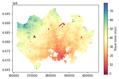
It is possible to enable legend for a geopandas plot by setting legend=True in the plotting parameters. If plotting the figure without a classification scheme you get a color bar as the legend item and it is easy to add a label for the legend using legend_kwds. You can read more about creating a legend via geopandas in here.

# Create one subplot. Control figure size in here.
fig, ax = plt.subplots(figsize=(6,4))

# Visualize the travel times into 9 classes using "Quantiles" classification scheme
grid.plot(ax=ax, column="car_r_t", 
          linewidth=0.03, 
          cmap="Spectral", 
          alpha=0.9, 
          legend=True, 
          legend_kwds={'label': "Travel time (min)"}
         )

#ax.get_legend().set_bbox_to_anchor(8)
#ax.get_legend().set_title("Legend title")

# Remove the empty white-space around the axes
plt.tight_layout()

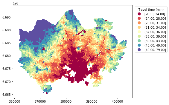
If plotting a map using a classification scheme, we get a different kind of ledend that shows the class values. In this case, we can control the position and title of the legend using matplotlib tools. We first need to access the Legend object and then change it’s properties.

# Create one subplot. Control figure size in here.
fig, ax = plt.subplots(figsize=(10,5))

# Visualize the travel times into 9 classes using "Quantiles" classification scheme
grid.plot(ax=ax, 
          column="car_r_t", 
          linewidth=0.03, 
          cmap="Spectral", 
          scheme="quantiles", 
          k=9, 
          legend=True, 
          )

# Re-position the legend and set a title
ax.get_legend().set_bbox_to_anchor((1.3,1))
ax.get_legend().set_title("Travel time (min)")

# Remove the empty white-space around the axes
plt.tight_layout()

You can read more info about adjusting legends in the matplotlig legend guide.

Adding basemap from external source#

It is often useful to add a basemap to your visualization that shows e.g. streets, placenames and other contextual information. This can be done easily by using ready-made background map tiles from different providers such as OpenStreetMap or Stamen Design. A Python library called contextily is a handy package that can be used to fetch geospatial raster files and add them to your maps. Map tiles are typically distributed in Web Mercator projection (EPSG:3857), hence it is often necessary to reproject all the spatial data into Web Mercator before visualizing the data.

In this tutorial, we will see how to add a basemap underneath our previous visualization.

Read in the travel time data:

import geopandas as gpd
import matplotlib.pyplot as plt
import contextily as ctx
%matplotlib inline

# Filepaths
grid_fp = "data/TravelTimes_to_5975375_RailwayStation.shp"

# Read data
grid = gpd.read_file(grid_fp)
grid.head(3)

	car_m_d	car_m_t	car_r_d	car_r_t	from_id	pt_m_d	pt_m_t	pt_m_tt	pt_r_d	pt_r_t	pt_r_tt	to_id	walk_d	walk_t	geometry
0	32297	43	32260	48	5785640	32616	116	147	32616	108	139	5975375	32164	459	POLYGON ((382000.000 6697750.000, 381750.000 6...
1	32508	43	32471	49	5785641	32822	119	145	32822	111	133	5975375	29547	422	POLYGON ((382250.000 6697750.000, 382000.000 6...
2	30133	50	31872	56	5785642	32940	121	146	32940	113	133	5975375	29626	423	POLYGON ((382500.000 6697750.000, 382250.000 6...

Check the input crs:

print(grid.crs)

epsg:3067

Reproject the layer to ESPG 3857 projection (Web Mercator):

# Reproject to EPSG 3857
data = grid.to_crs(epsg=3857)
print(data.crs)

epsg:3857

Now the crs is epsg:3857. Also the coordinate values in the geometry column have changed:

data.head(2)

	car_m_d	car_m_t	car_r_d	car_r_t	from_id	pt_m_d	pt_m_t	pt_m_tt	pt_r_d	pt_r_t	pt_r_tt	to_id	walk_d	walk_t	geometry
0	32297	43	32260	48	5785640	32616	116	147	32616	108	139	5975375	32164	459	POLYGON ((2767221.646 8489079.101, 2766716.966...
1	32508	43	32471	49	5785641	32822	119	145	32822	111	133	5975375	29547	422	POLYGON ((2767726.329 8489095.521, 2767221.646...

Next, we can plot our data using geopandas and add a basemap for our plot by using a function called add_basemap() from contextily:

# Control figure size in here
fig, ax = plt.subplots(figsize=(12,8))

# Plot the data
data.plot(ax=ax, column='pt_r_t', cmap='RdYlBu', linewidth=0, scheme="quantiles", k=9, alpha=0.6)

# Add basemap 
ctx.add_basemap(ax)

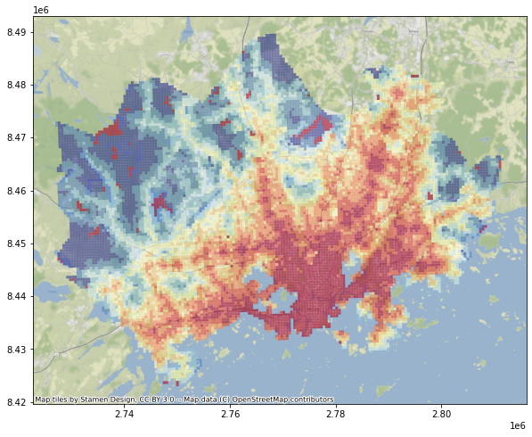
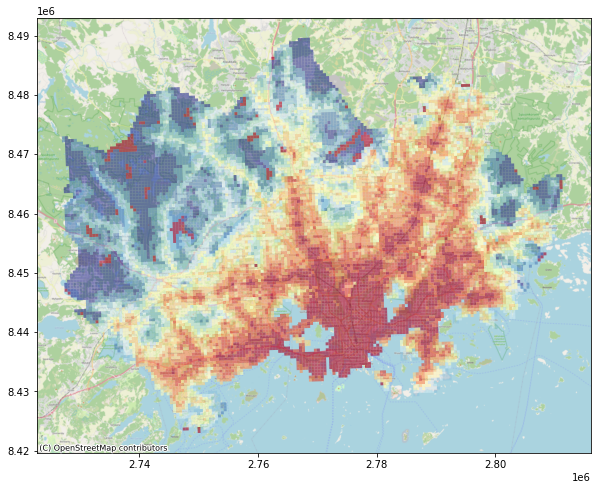
As we can see, now the map has a background map that is by default using the Stamen Terrain background from Stamen Design.

There are also various other possible data sources and styles for background maps.

Contextily’s tile_providers contain a list of providers and styles that can be used to control the appearence of your background map:

dir(ctx.providers)

['BasemapAT',
 'CartoDB',
 'Esri',
 'FreeMapSK',
 'GeoportailFrance',
 'HERE',
 'HikeBike',
 'Hydda',
 'JusticeMap',
 'MapBox',
 'MtbMap',
 'NASAGIBS',
 'NLS',
 'OneMapSG',
 'OpenFireMap',
 'OpenMapSurfer',
 'OpenPtMap',
 'OpenRailwayMap',
 'OpenSeaMap',
 'OpenStreetMap',
 'OpenTopoMap',
 'OpenWeatherMap',
 'SafeCast',
 'Stamen',
 'Thunderforest',
 'Wikimedia',
 'nlmaps']

There are multiple style options for most of these providers, for example:

ctx.providers.OpenStreetMap.keys()

dict_keys(['Mapnik', 'DE', 'CH', 'France', 'HOT', 'BZH'])

It is possible to change the tile provider using the source -parameter in add_basemap() function. Let’s see how we can change the bacground map as the basic OpenStreetMap background:

# Control figure size in here
fig, ax = plt.subplots(figsize=(12,8))

# Plot the data
data.plot(ax=ax, column='pt_r_t', cmap='RdYlBu', linewidth=0, scheme="quantiles", k=9, alpha=0.6)

# Add basemap with basic OpenStreetMap visualization
ctx.add_basemap(ax, source=ctx.providers.OpenStreetMap.Mapnik)

Let’s take a subset of our data to see a bit better the background map characteristics:

# Control figure size in here
fig, ax = plt.subplots(figsize=(12,8))

# Subset the data to seel only grid squares near the destination
subset = data.loc[(data['pt_r_t']>=0) & (data['pt_r_t']<=15)]

# Plot the data from subset
subset.plot(ax=ax, column='pt_r_t', cmap='RdYlBu', linewidth=0, scheme="quantiles", k=5, alpha=0.6)

# Add basemap with `OSM_A` style
ctx.add_basemap(ax, source=ctx.providers.OpenStreetMap.Mapnik)

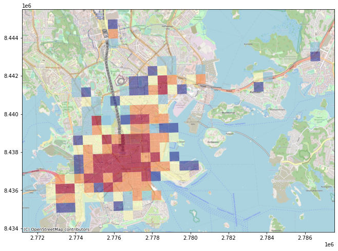
As we can see now our map has much more details in it as the zoom level of the background map is larger. By default contextily sets the zoom level automatically but it is possible to also control that manually using parameter zoom. The zoom level is by default specified as auto but you can control that by passing in zoom level as numbers ranging typically from 1 to 19 (the larger the number, the more details your basemap will have).

Let’s reduce the level of detail from our map by passing zoom=11:

# Control figure size in here
fig, ax = plt.subplots(figsize=(12,8))

# Plot the data from subset
subset.plot(ax=ax, column='pt_r_t', cmap='RdYlBu', linewidth=0, scheme="quantiles", k=5, alpha=0.6)

# Add basemap with `OSM_A` style using zoom level of 11
ctx.add_basemap(ax, zoom=11, source=ctx.providers.OpenStreetMap.Mapnik)

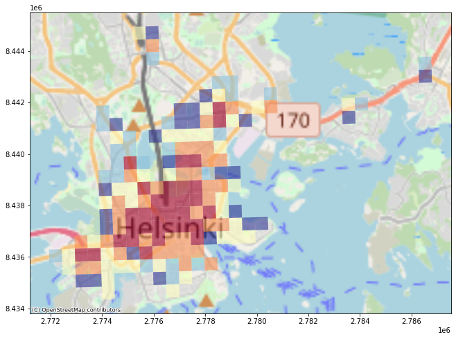
As we can see, the map has now less detail (a bit too blurry for such a small area).

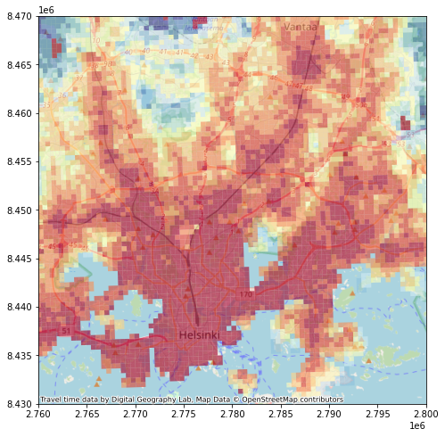
We can also use ax.set_xlim() and ax.set_ylim() -parameters to crop our map without altering the data. The parameters takes as input the coordinates for minimum and maximum on both axis (x and y). We can also change / remove the contribution text by using parameter attribution

Let’s add details about the data source, plot the original data, and crop the map:

credits = "Travel time data by Digital Geography Lab, Map Data © OpenStreetMap contributors"

# Control figure size in here
fig, ax = plt.subplots(figsize=(12,8))

# Plot the data
data.plot(ax=ax, column='pt_r_t', cmap='RdYlBu', linewidth=0, scheme="quantiles", k=9, alpha=0.6)

# Add basemap with `OSM_A` style using zoom level of 11 
# Modify the attribution 
ctx.add_basemap(ax, zoom=11, attribution=credits, source=ctx.providers.OpenStreetMap.Mapnik)

# Crop the figure
ax.set_xlim(2760000, 2800000)
ax.set_ylim(8430000, 8470000)

(8430000.0, 8470000.0)

It is also possible to use many other map tiles from different Tile Map Services as the background map. A good list of different available sources can be found from here. When using map tiles from different sources, it is necessary to parse a url address to the tile provider following a format defined by the provider.

Next, we will see how to use map tiles provided by CartoDB. To do that we need to parse the url address following their definition 'https://{s}.basemaps.cartocdn.com/{style}/{z}/{x}/{y}{scale}.png' where:

{s}: one of the available subdomains, either [a,b,c,d]
{z} : Zoom level. We support from 0 to 20 zoom levels in OSM tiling system.
{x},{y}: Tile coordinates in OSM tiling system
{scale}: OPTIONAL “@2x” for double resolution tiles
{style}: Map style, possible value is one of:
- light_all,
- dark_all,
- light_nolabels,
- light_only_labels,
- dark_nolabels,
- dark_only_labels,
- rastertiles/voyager,
- rastertiles/voyager_nolabels,
- rastertiles/voyager_only_labels,
- rastertiles/voyager_labels_under
We will use this information to parse the parameters in a way that contextily wants them:

# Control figure size in here
fig, ax = plt.subplots(figsize=(12,8))

# The formatting should follow: 'https://{s}.basemaps.cartocdn.com/{style}/{z}/{x}/{y}{scale}.png'
# Specify the style to use
style = "rastertiles/voyager"
cartodb_url = 'https://a.basemaps.cartocdn.com/%s/{z}/{x}/{y}.png' % style

# Plot the data from subset
subset.plot(ax=ax, column='pt_r_t', cmap='RdYlBu', linewidth=0, scheme="quantiles", k=5, alpha=0.6)
    
# Add basemap with `OSM_A` style using zoom level of 14 
ctx.add_basemap(ax, zoom=14, attribution="", source=cartodb_url)

# Crop the figure
ax.set_xlim(2770000, 2785000)
ax.set_ylim(8435000, 8442500)

(8435000.0, 8442500.0)

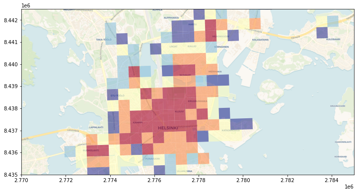
As we can see now we have yet again different kind of background map, now coming from CartoDB.

Let’s make a minor modification and change the style from "rastertiles/voyager" to "dark_all":

# Control figure size in here
fig, ax = plt.subplots(figsize=(12,8))

# The formatting should follow: 'https://{s}.basemaps.cartocdn.com/{style}/{z}/{x}/{y}{r}.png'
# Specify the style to use
style = "dark_all"
cartodb_url = 'https://a.basemaps.cartocdn.com/%s/{z}/{x}/{y}.png' % style

# Plot the data from subset
subset.plot(ax=ax, column='pt_r_t', cmap='RdYlBu', linewidth=0, scheme="quantiles", k=5, alpha=0.6)

# Add basemap with `OSM_A` style using zoom level of 14 
ctx.add_basemap(ax, zoom=13, attribution="", source=cartodb_url)

# Crop the figure
ax.set_xlim(2770000, 2785000)
ax.set_ylim(8435000, 8442500)

(8435000.0, 8442500.0)

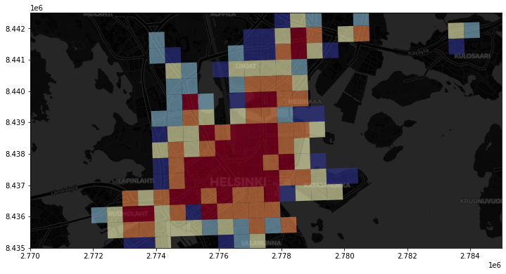
Great! Now we have dark background map fetched from CartoDB. In a similar manner, you can use any map tiles from various other tile providers such as the ones listed in leaflet-providers.

Static maps

Contents

Static maps#

Data#

Static maps in geopandas#

Adding a legend#

Adding basemap from external source#