Network analysis in Python
Contents
Network analysis in Python#
Finding a shortest path using a specific street network is a common GIS problem that has many practical applications. For example navigators are one of those “every-day” applications where routing using specific algorithms is used to find the optimal route between two (or multiple) points.
It is also possible to perform network analysis such as tranposrtation routing in Python. Networkx is a Python module that provides tools for analyzing networks in various different ways. It also contains algorithms such as Dijkstra’s algorithm or A* algoritm that are commonly used to find shortest paths along transportation network.
To be able to conduct network analysis, it is, of course, necessary to have a network that is used for the analyses. The OSMnx package enables us to retrieve routable networks from OpenStreetMap for various transport modes (walking, cycling and driving). OSMnx also combines some functionalities from networkx module to make it straightforward to conduct routing analysis based on OpenStreetMap data.
Next we will test the routing functionalities of OSMnx by finding a shortest path between two points based on drivable roads. With tiny modifications, it is also possible to repeat the analysis for the walkable street network.
Get the network#
Let’s again start by importing the required modules
import osmnx as ox
import networkx as nx
import geopandas as gpd
import matplotlib.pyplot as plt
import pandas as pd
from pyproj import CRS
import contextily as ctx
When fetching netowrk data from OpenStreetMap using OSMnx, it is possible to define the type of street network using the network_type parameter (see options from the OSMnx documentation).
Let’s download the OSM data from Kamppi but this only the bike network. If that does not work, try the driveable network (less roads, faster query..).
place_name = "Kamppi, Helsinki, Finland"
# Retrieve the network
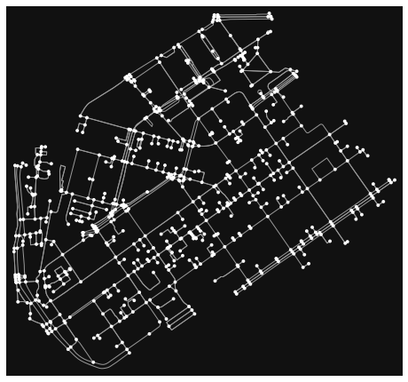
graph = ox.graph_from_place(place_name, network_type='bike')
# plot the graph:
fig, ax = ox.plot_graph(graph)
Pro tip! Sometimes the shortest path might go slightly outside the defined area of interest. To account for this, we can fetch the network for a bit larger area than the district of Kamppi, in case the shortest path is not completely inside its boundaries.
# Get the area of interest polygon
place_polygon = ox.geocode_to_gdf(place_name)
# Re-project the polygon to a local projected CRS
place_polygon = place_polygon.to_crs(epsg=3067)
# Buffer a bit
place_polygon["geometry"] = place_polygon.buffer(200)
# Re-project the polygon back to WGS84, as required by osmnx
place_polygon = place_polygon.to_crs(epsg=4326)
# Retrieve the network
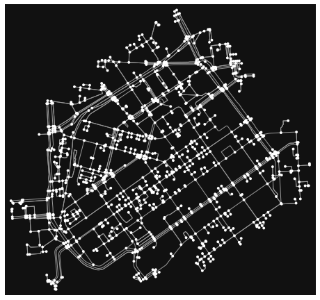
graph = ox.graph_from_polygon(place_polygon["geometry"].values[0], network_type='bike')
Plot the graph:
fig, ax = ox.plot_graph(graph)
Okey so now we have streets for the travel mode we specified earlier. Let’s have a colser look at the attributes of the street network. Easiest way to do this is to convert the graph (nodes and edges) into GeoDataFrames.
Converting graph into a GeoDataFrame can be done with function graph_to_gdfs() that we already used in previous tutorial. With parameters nodes and edges, it is possible to control whether to retrieve both nodes and edges from the graph.
# Retrieve only edges from the graph
edges = ox.graph_to_gdfs(graph, nodes=False, edges=True)
# Check columns
edges.columns
Index(['osmid', 'oneway', 'lanes', 'name', 'highway', 'maxspeed', 'length',
       'geometry', 'access', 'bridge', 'junction', 'tunnel', 'service', 'u',
       'v', 'key'],
      dtype='object')
# Check crs
edges.crs
<Geographic 2D CRS: EPSG:4326>
Name: WGS 84
Axis Info [ellipsoidal]:
- Lat[north]: Geodetic latitude (degree)
- Lon[east]: Geodetic longitude (degree)
Area of Use:
- name: World
- bounds: (-180.0, -90.0, 180.0, 90.0)
Datum: World Geodetic System 1984
- Ellipsoid: WGS 84
- Prime Meridian: Greenwich
Note that the CRS of the GeoDataFrame is be WGS84 (epsg: 4326).
edges.head()
| osmid | oneway | lanes | name | highway | maxspeed | length | geometry | access | bridge | junction | tunnel | service | u | v | key | |
|---|---|---|---|---|---|---|---|---|---|---|---|---|---|---|---|---|
| 0 | 23717777 | True | 2 | Porkkalankatu | primary | 40 | 10.404 | LINESTRING (24.92106 60.16479, 24.92087 60.16479) | NaN | NaN | NaN | NaN | NaN | 25216594 | 1372425721 | 0 |
| 1 | 23856784 | True | 2 | Mechelininkatu | primary | 40 | 40.885 | LINESTRING (24.92106 60.16479, 24.92095 60.164... | NaN | NaN | NaN | NaN | NaN | 25216594 | 1372425714 | 0 |
| 2 | [59355210, 4229487] | False | 2 | Santakatu | residential | 30 | 44.310 | LINESTRING (24.91994 60.16279, 24.91932 60.162... | NaN | NaN | NaN | NaN | NaN | 25238865 | 146447626 | 0 |
| 3 | 7842621 | False | NaN | Sinikaislankuja | residential | 30 | 76.704 | LINESTRING (24.91994 60.16279, 24.91995 60.162... | NaN | NaN | NaN | NaN | NaN | 25238865 | 57661989 | 0 |
| 4 | 231643806 | False | NaN | NaN | cycleway | NaN | 59.812 | LINESTRING (24.91994 60.16279, 24.92014 60.162... | NaN | NaN | NaN | NaN | NaN | 25238865 | 314767800 | 0 |
Okey, so we have quite many columns in our GeoDataFrame. Most of the columns are fairly self-explanatory but the following table describes all of them.
Most of the attributes come directly from the OpenStreetMap, however, columns u and v are Networkx specific ids. You can click on the links to get more information about each attribute:
Column |
Description |
Data type |
|---|---|---|
Bridge feature |
boolean |
|
geometry |
Geometry of the feature |
Shapely.geometry |
Tag for roads (road type) |
str / list |
|
Number of lanes |
int (or nan) |
|
Length of feature (meters) |
float |
|
maximum legal speed limit |
int /list |
|
Name of the (street) element |
str (or nan) |
|
One way road |
boolean |
|
Unique ids for the element |
list |
|
The first node of edge |
int |
|
The last node of edge |
int |
Let’s take a look what kind of features we have in the highway column:
edges['highway'].value_counts()
---------------------------------------------------------------------------
TypeError                                 Traceback (most recent call last)
pandas/_libs/hashtable_class_helper.pxi in pandas._libs.hashtable.PyObjectHashTable.map_locations()

TypeError: unhashable type: 'list'
Exception ignored in: 'pandas._libs.index.IndexEngine._call_map_locations'
Traceback (most recent call last):
  File "pandas/_libs/hashtable_class_helper.pxi", line 1709, in pandas._libs.hashtable.PyObjectHashTable.map_locations
TypeError: unhashable type: 'list'
service                      873
cycleway                     484
residential                  466
tertiary                     217
primary                      164
pedestrian                   134
secondary                    121
unclassified                  42
living_street                 16
[living_street, service]       6
[residential, cycleway]        6
[pedestrian, residential]      4
tertiary_link                  2
[pedestrian, service]          2
[pedestrian, cycleway]         2
primary_link                   1
[unclassified, service]        1
Name: highway, dtype: int64
I now we can confirm that as a result our street network indeed only contains such streets where it is allowed to drive with a car as there are no e.g. cycleways or footways included in the data.
As the data is in WGS84 format, we might want to reproject our data into a metric system before proceeding to the shortest path analysis. We can re-project the graph from latitudes and longitudes to an appropriate UTM zone using the project_graph() function from OSMnx.
# Project the data
graph_proj = ox.project_graph(graph)
# Get Edges and Nodes
nodes_proj, edges_proj = ox.graph_to_gdfs(graph_proj, nodes=True, edges=True)
print("Coordinate system:", edges_proj.crs)
Coordinate system: +proj=utm +zone=35 +ellps=WGS84 +datum=WGS84 +units=m +no_defs +type=crs
edges_proj.head()
| osmid | oneway | lanes | name | highway | maxspeed | length | geometry | access | bridge | junction | tunnel | service | u | v | key | |
|---|---|---|---|---|---|---|---|---|---|---|---|---|---|---|---|---|
| 0 | 23717777 | True | 2 | Porkkalankatu | primary | 40 | 10.404 | LINESTRING (384631.322 6671580.071, 384620.884... | NaN | NaN | NaN | NaN | NaN | 25216594 | 1372425721 | 0 |
| 1 | 23856784 | True | 2 | Mechelininkatu | primary | 40 | 40.885 | LINESTRING (384631.322 6671580.071, 384624.750... | NaN | NaN | NaN | NaN | NaN | 25216594 | 1372425714 | 0 |
| 2 | [59355210, 4229487] | False | 2 | Santakatu | residential | 30 | 44.310 | LINESTRING (384562.162 6671358.993, 384527.710... | NaN | NaN | NaN | NaN | NaN | 25238865 | 146447626 | 0 |
| 3 | 7842621 | False | NaN | Sinikaislankuja | residential | 30 | 76.704 | LINESTRING (384562.162 6671358.993, 384562.951... | NaN | NaN | NaN | NaN | NaN | 25238865 | 57661989 | 0 |
| 4 | 231643806 | False | NaN | NaN | cycleway | NaN | 59.812 | LINESTRING (384562.162 6671358.993, 384573.361... | NaN | NaN | NaN | NaN | NaN | 25238865 | 314767800 | 0 |
Okey, as we can see from the CRS the data is now in UTM projection using zone 35 which is the one used for Finland, and indeed the orientation of the map and the geometry values also confirm this.
Furthermore, we can check the epsg code of this projection using pyproj CRS:
CRS(edges_proj.crs).to_epsg()
32635
Indeed, the projection is now WGS 84 / UTM zone 35N, EPSG:32635.
Analyzing the network properties#
Now as we have seen some of the basic functionalities of OSMnx such as downloading the data and converting data from graph to GeoDataFrame, we can take a look some of the analytical features of omsnx. Osmnx includes many useful functionalities to extract information about the network.
To calculate some of the basic street network measures we can use basic_stats() function in OSMnx:
# Calculate network statistics
stats = ox.basic_stats(graph_proj, circuity_dist='euclidean')
stats
{'n': 1182,
 'm': 2541,
 'k_avg': 4.299492385786802,
 'intersection_count': 865,
 'streets_per_node_avg': 2.6996615905245345,
 'streets_per_node_counts': {0: 0, 1: 317, 2: 16, 3: 572, 4: 259, 5: 18},
 'streets_per_node_proportion': {0: 0.0,
  1: 0.26818950930626057,
  2: 0.01353637901861252,
  3: 0.48392554991539766,
  4: 0.21912013536379019,
  5: 0.015228426395939087},
 'edge_length_total': 90784.85899999987,
 'edge_length_avg': 35.72800432900428,
 'street_length_total': 56745.758000000016,
 'street_length_avg': 36.49244887459808,
 'street_segments_count': 1555,
 'node_density_km': None,
 'intersection_density_km': None,
 'edge_density_km': None,
 'street_density_km': None,
 'circuity_avg': 1.0452946617747503,
 'self_loop_proportion': 0.0015741833923652105,
 'clean_intersection_count': None,
 'clean_intersection_density_km': None}
To be able to extract the more advanced statistics (and some of the missing ones above) from the street network, it is required to have information about the coverage area of the network. Let’s calculate the area of the convex hull of the street network and see what we can get.
# Get the Convex Hull of the network
convex_hull = edges_proj.unary_union.convex_hull

# Show output
convex_hull

Now we can use the Convex Hull above to calculate extended statistics for the network. As some of the metrics are produced separately for each node, they produce a lot of output. Here, we combine the basic and extended statistics into one pandas Series to keep things in more compact form.
# Calculate the area
area = convex_hull.area

# Calculate statistics with density information
stats = ox.basic_stats(graph_proj, area=area)
extended_stats = ox.extended_stats(graph_proj, ecc=True, cc=True)

# Add extened statistics to the basic statistics
for key, value in extended_stats.items():
    stats[key] = value

# Convert the dictionary to a Pandas series for a nicer output
pd.Series(stats)
n                                                                                   1182
m                                                                                   2541
k_avg                                                                            4.29949
intersection_count                                                                   865
streets_per_node_avg                                                             2.69966
streets_per_node_counts                     {0: 0, 1: 317, 2: 16, 3: 572, 4: 259, 5: 18}
streets_per_node_proportion            {0: 0.0, 1: 0.26818950930626057, 2: 0.01353637...
edge_length_total                                                                90784.9
edge_length_avg                                                                   35.728
street_length_total                                                              56745.8
street_length_avg                                                                36.4924
street_segments_count                                                               1555
node_density_km                                                                  685.441
intersection_density_km                                                          501.613
edge_density_km                                                                  52646.1
street_density_km                                                                32906.8
circuity_avg                                                                 1.19914e-05
self_loop_proportion                                                          0.00157418
clean_intersection_count                                                            None
clean_intersection_density_km                                                       None
avg_neighbor_degree                    {25216594: 2.0, 25238865: 2.3333333333333335, ...
avg_neighbor_degree_avg                                                          2.51369
avg_weighted_neighbor_degree           {25216594: 0.07798943243190548, 25238865: 0.03...
avg_weighted_neighbor_degree_avg                                                0.140427
degree_centrality                      {25216594: 0.004233700254022015, 25238865: 0.0...
degree_centrality_avg                                                         0.00364055
clustering_coefficient                 {25216594: 0.1, 25238865: 0, 25238874: 0.16666...
clustering_coefficient_avg                                                     0.0438804
clustering_coefficient_weighted        {25216594: 0.003767020492241665, 25238865: 0, ...
clustering_coefficient_weighted_avg                                           0.00191556
pagerank                               {25216594: 0.0011399168859237627, 25238865: 0....
pagerank_max_node                                                             9255772098
pagerank_max                                                                  0.00410893
pagerank_min_node                                                               60546333
pagerank_min                                                                 0.000127733
eccentricity                           {25216594: 2115.77, 25238865: 1992.49400000000...
diameter                                                                         2477.63
radius                                                                           1247.75
center                                                                      [7698539437]
periphery                                                                   [8324096500]
closeness_centrality                   {25216594: 0.0009553219974087529, 25238865: 0....
closeness_centrality_avg                                                      0.00107821
dtype: object
As we can see, now we have a LOT of information about our street network that can be used to understand its structure. We can for example see that the average node density in our network is 149 nodes/km and that the total edge length of our network is almost 20 kilometers.
Furthermore, we can see that the degree centrality of our network is on average 0.0326515. Degree is a simple centrality measure that counts how many neighbors a node has (here a fraction of nodes it is connected to). Another interesting measure is the PageRank that measures the importance of specific node in the graph. Here we can see that the most important node in our graph seem to a node with osmid 25416262. PageRank was the algorithm that Google first developed (Larry Page & Sergei Brin) to order the search engine results and became famous for.
You can read the Wikipedia article about different centrality measures if you are interested what the other centrality measures mean.
Shortest path analysis#
Let’s now calculate the shortest path between two points using the shortest path function in Networkx.
Origin and destination points#
First we need to specify the source and target locations for our route. If you are familiar with the Kamppi area, you can specify a custom placename as a source location. Or, you can follow along and choose these points as the origin and destination in the analysis:
Maria 01 - and old hospital area and current startup hub.
ruttopuisto - a park. Official name of this park is “Vanha kirkkopuisto”, but nominatim is also able to geocode the nickname.
We could figure out the coordinates for these locations manually, and create shapely points based on the coordinates. However, it is more handy to fetch the location of our source destination directly from OSM:
# Set place name
placename = "Maria 01, Helsinki"
# Geocode the place name
geocoded_place = ox.geocode_to_gdf(placename)
# Check the result
geocoded_place
| geometry | place_name | bbox_north | bbox_south | bbox_east | bbox_west | |
|---|---|---|---|---|---|---|
| 0 | POLYGON ((24.92122 60.16644, 24.92126 60.16625... | Maria 01, Mechelininkatu, Hietalahti, Kamppi, ... | 60.167525 | 60.16624 | 24.92317 | 24.921221 |
As output, we received the building footprint. From here, we can get the centroid as the source location of our shortest path analysis. However, we first need to project the data into the correct crs:
# Re-project into the same CRS as the road network
geocoded_place = geocoded_place.to_crs(CRS(edges_proj.crs))
# Get centroid as shapely point
origin = geocoded_place["geometry"].centroid.values[0]
print(origin)
POINT (384692.1787195496 6671817.486579246)
Great! Now we have defined the origin point for our network analysis. We can repeat the same steps to retrieve central point of ruttopuisto-park as the destination:
# Set place name
placename = "ruttopuisto"

# Geocode the place name
geocoded_place = ox.geocode_to_gdf(placename)

# Re-project into the same CRS as the road network
geocoded_place = geocoded_place.to_crs(CRS(edges_proj.crs))

# Get centroid of the polygon as shapely point
destination = geocoded_place["geometry"].centroid.values[0]

print(destination)
POINT (385673.4277923346 6671690.223032337)
Now we have shapely points representing the origin and destination locations for our network analysis. Next step is to find these points on the routable network before the final routing.
Nearest node#
Let’s now find the nearest graph nodes (and their node IDs) to these points using OSMnx get_nearest_node. As a starting point, we have the two Shapely Point objects we just defined as the origin and destination locations.
According to the documentation of this function, we need to parse Point coordinates as coordinate-tuples in this order: latitude, longitude(or y, x). As our data is now projected to UTM projection, we need to specify with method parameter that the function uses 'euclidean' distances to calculate the distance from the point to the closest node (with decimal derees, use 'haversine', which determines the great-circle distances). The method parameter is important if you want to know the actual distance between the Point and the closest node which you can retrieve by specifying parameter return_dist=True.
# Get origin x and y coordinates
orig_xy = (origin.y, origin.x)

# Get target x and y coordinates
target_xy = (destination.y, destination.x)
# Find the node in the graph that is closest to the origin point (here, we want to get the node id)
orig_node_id = ox.get_nearest_node(graph_proj, orig_xy, method='euclidean')
orig_node_id
319719983
# Find the node in the graph that is closest to the target point (here, we want to get the node id)
target_node_id = ox.get_nearest_node(graph_proj, target_xy, method='euclidean')
target_node_id
1377208998
Now we have the IDs for the closest nodes that were found from the graph to the origin and target points that we specified.
Let’s retrieve the node information from the nodes_proj GeoDataFrame by passing the ids to the loc indexer
# Retrieve the rows from the nodes GeoDataFrame based on the node id (node id is the index label)
orig_node = nodes_proj.loc[orig_node_id]
target_node = nodes_proj.loc[target_node_id]
Let’s also create a GeoDataFrame that contains these points
# Create a GeoDataFrame from the origin and target points
od_nodes = gpd.GeoDataFrame([orig_node, target_node], geometry='geometry', crs=nodes_proj.crs)
od_nodes.head()
| y | x | osmid | lon | lat | highway | ref | geometry | |
|---|---|---|---|---|---|---|---|---|
| 319719983 | 6.671816e+06 | 384706.296089 | 319719983 | 24.922273 | 60.166932 | NaN | NaN | POINT (384706.296 6671815.989) |
| 1377208998 | 6.671730e+06 | 385612.532846 | 1377208998 | 24.938641 | 60.166412 | NaN | NaN | POINT (385612.533 6671729.630) |
Okay, as a result we got now the closest node IDs of our origin and target locations. As you can see, the index in this GeoDataFrame corresponds to the IDs that we found with get_nearest_node() function.
Routing#
Now we are ready to do the routing and find the shortest path between the origin and target locations
by using the shortest_path() function of networkx.
With weight -parameter we can specify that 'length' attribute should be used as the cost impedance in the routing. If specifying the weight parameter, NetworkX will use by default Dijkstra’s algorithm to find the optimal route. We need to specify the graph that is used for routing, and the origin ID (source) and the target ID in between the shortest path will be calculated:
# Calculate the shortest path
route = nx.shortest_path(G=graph_proj, source=orig_node_id, target=target_node_id, weight='length')

# Show what we have
print(route)
[319719983, 1382316822, 1382316829, 1382316852, 5464887863, 1382320461, 5154747161, 1378064352, 1372461709, 1372441203, 3205236795, 3205236793, 8244768393, 60278325, 56115897, 60072524, 7699019923, 7699019916, 7699019908, 7699019903, 267117319, 1897461604, 724233143, 724233128, 267117317, 846597945, 846597947, 2037356632, 1547012339, 569742461, 1372441189, 4524927399, 298372061, 7702074840, 7702074833, 60170471, 8856704555, 3227176325, 7676757030, 8856704573, 7676756995, 8856704588, 1377211668, 60170470, 8874925445, 3228706311, 1377211669, 1377209035, 1377208998]
As a result we get a list of all the nodes that are along the shortest path.
We could extract the locations of those nodes from the
nodes_projGeoDataFrame and create a LineString presentation of the points, but luckily, OSMnx can do that for us and we can plot shortest path by usingplot_graph_route()function:
# Plot the shortest path
fig, ax = ox.plot_graph_route(graph_proj, route)
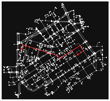
Nice! Now we have the shortest path between our origin and target locations. Being able to analyze shortest paths between locations can be valuable information for many applications. Here, we only analyzed the shortest paths based on distance but quite often it is more useful to find the optimal routes between locations based on the travelled time. Here, for example we could calculate the time that it takes to cross each road segment by dividing the length of the road segment with the speed limit and calculate the optimal routes by taking into account the speed limits as well that might alter the result especially on longer trips than here.
Saving shortest paths to disk#
Quite often you need to save the route into a file for further analysis and visualization purposes, or at least have it as a GeoDataFrame object in Python. Hence, let’s continue still a bit and see how we can turn the route into a linestring and save the shortest path geometry and related attributes into a geopackage file.
First we need to get the nodes that belong to the shortest path:
# Get the nodes along the shortest path
route_nodes = nodes_proj.loc[route]
route_nodes
| y | x | osmid | lon | lat | highway | ref | geometry | |
|---|---|---|---|---|---|---|---|---|
| 319719983 | 6.671816e+06 | 384706.296089 | 319719983 | 24.922273 | 60.166932 | NaN | NaN | POINT (384706.296 6671815.989) |
| 1382316822 | 6.671839e+06 | 384709.579017 | 1382316822 | 24.922319 | 60.167142 | NaN | NaN | POINT (384709.579 6671839.311) |
| 1382316829 | 6.671850e+06 | 384711.044607 | 1382316829 | 24.922339 | 60.167236 | NaN | NaN | POINT (384711.045 6671849.707) |
| 1382316852 | 6.671861e+06 | 384712.504583 | 1382316852 | 24.922359 | 60.167338 | NaN | NaN | POINT (384712.505 6671860.984) |
| 5464887863 | 6.671865e+06 | 384713.220293 | 5464887863 | 24.922370 | 60.167377 | NaN | NaN | POINT (384713.220 6671865.374) |
| 1382320461 | 6.671887e+06 | 384719.671826 | 1382320461 | 24.922473 | 60.167575 | NaN | NaN | POINT (384719.672 6671887.215) |
| 5154747161 | 6.671874e+06 | 384758.946564 | 5154747161 | 24.923188 | 60.167471 | NaN | NaN | POINT (384758.947 6671874.411) |
| 1378064352 | 6.671869e+06 | 384776.322613 | 1378064352 | 24.923504 | 60.167428 | NaN | NaN | POINT (384776.323 6671869.117) |
| 1372461709 | 6.671853e+06 | 384830.142058 | 1372461709 | 24.924482 | 60.167300 | NaN | NaN | POINT (384830.142 6671853.149) |
| 1372441203 | 6.671833e+06 | 384899.781649 | 1372441203 | 24.925748 | 60.167135 | NaN | NaN | POINT (384899.782 6671832.539) |
| 3205236795 | 6.671821e+06 | 384940.404180 | 3205236795 | 24.926486 | 60.167040 | NaN | NaN | POINT (384940.404 6671820.709) |
| 3205236793 | 6.671819e+06 | 384945.256772 | 3205236793 | 24.926574 | 60.167029 | NaN | NaN | POINT (384945.257 6671819.264) |
| 8244768393 | 6.671819e+06 | 384946.335048 | 8244768393 | 24.926594 | 60.167026 | NaN | NaN | POINT (384946.335 6671818.940) |
| 60278325 | 6.671811e+06 | 384973.265328 | 60278325 | 24.927083 | 60.166961 | crossing | NaN | POINT (384973.265 6671810.884) |
| 56115897 | 6.671809e+06 | 384980.951995 | 56115897 | 24.927223 | 60.166943 | traffic_signals | NaN | POINT (384980.952 6671808.614) |
| 60072524 | 6.671806e+06 | 384989.084898 | 60072524 | 24.927371 | 60.166924 | crossing | NaN | POINT (384989.085 6671806.231) |
| 7699019923 | 6.671802e+06 | 385004.619120 | 7699019923 | 24.927653 | 60.166886 | NaN | NaN | POINT (385004.619 6671801.508) |
| 7699019916 | 6.671787e+06 | 385053.438353 | 7699019916 | 24.928540 | 60.166771 | NaN | NaN | POINT (385053.438 6671787.182) |
| 7699019908 | 6.671778e+06 | 385082.009990 | 7699019908 | 24.929060 | 60.166698 | NaN | NaN | POINT (385082.010 6671778.150) |
| 7699019903 | 6.671771e+06 | 385104.890696 | 7699019903 | 24.929476 | 60.166640 | NaN | NaN | POINT (385104.891 6671770.925) |
| 267117319 | 6.671765e+06 | 385122.997863 | 267117319 | 24.929805 | 60.166595 | NaN | NaN | POINT (385122.998 6671765.364) |
| 1897461604 | 6.671758e+06 | 385124.328076 | 1897461604 | 24.929834 | 60.166527 | crossing | NaN | POINT (385124.328 6671757.666) |
| 724233143 | 6.671751e+06 | 385129.242187 | 724233143 | 24.929926 | 60.166471 | NaN | NaN | POINT (385129.242 6671751.271) |
| 724233128 | 6.671747e+06 | 385134.459142 | 724233128 | 24.930022 | 60.166435 | NaN | NaN | POINT (385134.459 6671747.096) |
| 267117317 | 6.671744e+06 | 385154.958400 | 267117317 | 24.930393 | 60.166409 | NaN | NaN | POINT (385154.958 6671743.611) |
| 846597945 | 6.671741e+06 | 385157.556336 | 846597945 | 24.930441 | 60.166384 | NaN | NaN | POINT (385157.556 6671740.744) |
| 846597947 | 6.671741e+06 | 385168.666425 | 846597947 | 24.930642 | 60.166387 | NaN | NaN | POINT (385168.666 6671740.674) |
| 2037356632 | 6.671745e+06 | 385172.125438 | 2037356632 | 24.930701 | 60.166429 | NaN | NaN | POINT (385172.125 6671745.257) |
| 1547012339 | 6.671745e+06 | 385191.531754 | 1547012339 | 24.931051 | 60.166433 | NaN | NaN | POINT (385191.532 6671745.173) |
| 569742461 | 6.671734e+06 | 385229.630826 | 569742461 | 24.931743 | 60.166343 | NaN | NaN | POINT (385229.631 6671733.927) |
| 1372441189 | 6.671719e+06 | 385268.523844 | 1372441189 | 24.932452 | 60.166218 | NaN | NaN | POINT (385268.524 6671718.767) |
| 4524927399 | 6.671723e+06 | 385274.647756 | 4524927399 | 24.932560 | 60.166256 | NaN | NaN | POINT (385274.648 6671722.799) |
| 298372061 | 6.671664e+06 | 385321.073501 | 298372061 | 24.933429 | 60.165737 | NaN | NaN | POINT (385321.074 6671663.529) |
| 7702074840 | 6.671673e+06 | 385336.128259 | 7702074840 | 24.933695 | 60.165830 | NaN | NaN | POINT (385336.128 6671673.444) |
| 7702074833 | 6.671687e+06 | 385356.847665 | 7702074833 | 24.934060 | 60.165959 | NaN | NaN | POINT (385356.848 6671687.094) |
| 60170471 | 6.671704e+06 | 385382.616738 | 60170471 | 24.934515 | 60.166117 | NaN | NaN | POINT (385382.617 6671703.996) |
| 8856704555 | 6.671723e+06 | 385411.444462 | 8856704555 | 24.935023 | 60.166293 | NaN | NaN | POINT (385411.444 6671722.641) |
| 3227176325 | 6.671725e+06 | 385414.610525 | 3227176325 | 24.935079 | 60.166311 | NaN | NaN | POINT (385414.611 6671724.615) |
| 7676757030 | 6.671750e+06 | 385453.325086 | 7676757030 | 24.935762 | 60.166546 | NaN | NaN | POINT (385453.325 6671749.549) |
| 8856704573 | 6.671755e+06 | 385462.274213 | 8856704573 | 24.935920 | 60.166600 | NaN | NaN | POINT (385462.274 6671755.321) |
| 7676756995 | 6.671765e+06 | 385477.769273 | 7676756995 | 24.936194 | 60.166694 | NaN | NaN | POINT (385477.769 6671765.312) |
| 8856704588 | 6.671777e+06 | 385495.230414 | 8856704588 | 24.936502 | 60.166800 | NaN | NaN | POINT (385495.230 6671776.557) |
| 1377211668 | 6.671789e+06 | 385514.573340 | 1377211668 | 24.936843 | 60.166917 | NaN | NaN | POINT (385514.573 6671789.024) |
| 60170470 | 6.671875e+06 | 385648.626456 | 60170470 | 24.939208 | 60.167730 | NaN | NaN | POINT (385648.626 6671875.418) |
| 8874925445 | 6.671847e+06 | 385666.360274 | 8874925445 | 24.939544 | 60.167484 | NaN | NaN | POINT (385666.360 6671847.394) |
| 3228706311 | 6.671822e+06 | 385682.863245 | 3228706311 | 24.939855 | 60.167257 | NaN | NaN | POINT (385682.863 6671821.559) |
| 1377211669 | 6.671789e+06 | 385703.651424 | 1377211669 | 24.940248 | 60.166968 | traffic_signals | NaN | POINT (385703.651 6671788.715) |
| 1377209035 | 6.671762e+06 | 385662.674736 | 1377209035 | 24.939525 | 60.166719 | NaN | NaN | POINT (385662.675 6671762.222) |
| 1377208998 | 6.671730e+06 | 385612.532846 | 1377208998 | 24.938641 | 60.166412 | NaN | NaN | POINT (385612.533 6671729.630) |
As we can see, now we have all the nodes that were part of the shortest path as a GeoDataFrame.
Now we can create a LineString out of the Point geometries of the nodes:
from shapely.geometry import LineString, Point

# Create a geometry for the shortest path
route_line = LineString(list(route_nodes.geometry.values))
route_line

Now we have the route as a LineString geometry.
Let’s make a GeoDataFrame out of it having some useful information about our route such as a list of the osmids that are part of the route and the length of the route.
# Create a GeoDataFrame
route_geom = gpd.GeoDataFrame([[route_line]], geometry='geometry', crs=edges_proj.crs, columns=['geometry'])

# Add a list of osmids associated with the route
route_geom.loc[0, 'osmids'] = str(list(route_nodes['osmid'].values))

# Calculate the route length
route_geom['length_m'] = route_geom.length

route_geom.head()
| geometry | osmids | length_m | |
|---|---|---|---|
| 0 | LINESTRING (384706.296 6671815.989, 384709.579... | [319719983, 1382316822, 1382316829, 1382316852... | 1342.967643 |
Now we have a GeoDataFrame that we can save to disk. Let’s still confirm that everything is ok by plotting our route on top of our street network and some buildings, and plot also the origin and target points on top of our map.
Get buildings:
tags = {'building': True}
buildings = ox.geometries_from_place(place_name, tags)
re-project buildings
buildings_proj = buildings.to_crs(CRS(edges_proj.crs))
/opt/conda/lib/python3.8/site-packages/ipykernel/ipkernel.py:287: DeprecationWarning: `should_run_async` will not call `transform_cell` automatically in the future. Please pass the result to `transformed_cell` argument and any exception that happen during thetransform in `preprocessing_exc_tuple` in IPython 7.17 and above.
  and should_run_async(code)
Let’s now plot the route and the street network elements to verify that everything is as it should:
fig, ax = plt.subplots(figsize=(12,8))

# Plot edges and nodes
edges_proj.plot(ax=ax, linewidth=0.75, color='gray')
nodes_proj.plot(ax=ax, markersize=2, color='gray')

# Add buildings
ax = buildings_proj.plot(ax=ax, facecolor='lightgray', alpha=0.7)

# Add the route
ax = route_geom.plot(ax=ax, linewidth=2, linestyle='--', color='red')

# Add the origin and destination nodes of the route
ax = od_nodes.plot(ax=ax, markersize=30, color='red')

# Add basemap
ctx.add_basemap(ax, crs=buildings_proj.crs, source=ctx.providers.CartoDB.Positron)
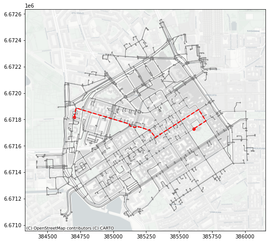
Great everything seems to be in order! As you can see, now we have a full control of all the elements of our map and we can use all the aesthetic properties that matplotlib provides to modify how our map will look like. Now we are almost ready to save our data into disk.
Prepare data for saving to file#
The data contain certain data types (such as list or boolean) that should be converted into character strings prior to saving the data to file.Another option would be to drop invalid columns.
edges_proj.head()
/opt/conda/lib/python3.8/site-packages/ipykernel/ipkernel.py:287: DeprecationWarning: `should_run_async` will not call `transform_cell` automatically in the future. Please pass the result to `transformed_cell` argument and any exception that happen during thetransform in `preprocessing_exc_tuple` in IPython 7.17 and above.
  and should_run_async(code)
| osmid | oneway | lanes | name | highway | maxspeed | length | geometry | access | bridge | junction | tunnel | service | u | v | key | |
|---|---|---|---|---|---|---|---|---|---|---|---|---|---|---|---|---|
| 0 | 23717777 | True | 2 | Porkkalankatu | primary | 40 | 10.404 | LINESTRING (384631.322 6671580.071, 384620.884... | NaN | NaN | NaN | NaN | NaN | 25216594 | 1372425721 | 0 |
| 1 | 23856784 | True | 2 | Mechelininkatu | primary | 40 | 40.885 | LINESTRING (384631.322 6671580.071, 384624.750... | NaN | NaN | NaN | NaN | NaN | 25216594 | 1372425714 | 0 |
| 2 | [59355210, 4229487] | False | 2 | Santakatu | residential | 30 | 44.310 | LINESTRING (384562.162 6671358.993, 384527.710... | NaN | NaN | NaN | NaN | NaN | 25238865 | 146447626 | 0 |
| 3 | 7842621 | False | NaN | Sinikaislankuja | residential | 30 | 76.704 | LINESTRING (384562.162 6671358.993, 384562.951... | NaN | NaN | NaN | NaN | NaN | 25238865 | 57661989 | 0 |
| 4 | 231643806 | False | NaN | NaN | cycleway | NaN | 59.812 | LINESTRING (384562.162 6671358.993, 384573.361... | NaN | NaN | NaN | NaN | NaN | 25238865 | 314767800 | 0 |
# Check if columns contain any list values
(edges_proj.applymap(type) == list).any()
/opt/conda/lib/python3.8/site-packages/ipykernel/ipkernel.py:287: DeprecationWarning: `should_run_async` will not call `transform_cell` automatically in the future. Please pass the result to `transformed_cell` argument and any exception that happen during thetransform in `preprocessing_exc_tuple` in IPython 7.17 and above.
  and should_run_async(code)
osmid        True
oneway      False
lanes        True
name         True
highway      True
maxspeed     True
length      False
geometry    False
access      False
bridge      False
junction    False
tunnel      False
service      True
u           False
v           False
key         False
dtype: bool
# Columns with invalid values
invalid_cols = ['lanes', 'maxspeed', 'name', 'oneway', 'osmid', "highway", "service"]

#  convert selected columns to string format
edges_proj[invalid_cols] = edges_proj[invalid_cols].astype(str)
# Check again if columns contain any list values
(edges_proj.applymap(type) == list).any()
osmid       False
oneway      False
lanes       False
name        False
highway     False
maxspeed    False
length      False
geometry    False
access      False
bridge      False
junction    False
tunnel      False
service     False
u           False
v           False
key         False
dtype: bool
Now we can see that most of the attributes are of type object that quite often (such as ours here) refers to a string type of data.
Save the data:#
import os

# Parse the place name for the output file names (replace spaces with underscores and remove commas)
place_name_out = place_name.replace(' ', '_').replace(',','')

# Output directory
out_dir = "data"

# Create output fp for a geopackage
out_fp = os.path.join(out_dir, f"OSM_{place_name_out}.gpkg")

# Save files
edges_proj.to_file(out_fp, layer="streets", driver="GPKG")
route_geom.to_file(out_fp, layer="route", driver="GPKG")
nodes_proj.to_file(out_fp, layer="nodes", driver="GPKG")
od_nodes.to_file(out_fp, layer="route_OD", driver="GPKG")
buildings[['geometry', 'name', 'addr:street']].to_file(out_fp, layer="buildings", driver="GPKG")
Great, now we have saved all the data that was used to produce the maps into a geopackage.
Advanced reading#
Here we learned how to solve a simple routing task between origin and destination points. What about if we have hundreads or thousands of origins? This is the case if you want to explore the travel distances to a spesific location across the whole city, for example, when analyzing the accessibility of jobs and services (like in the Travel Time Matrix dataset used in previous sections).
Check out pyrosm documentation on working with graphs for more advanced examples of network analysis in python. For example, pandana is a fast and efficient python library for creating aggretated network analysis in no time across large networks, and pyrosm can be used for preparing the input data for such analysis.