Processing toolbox scripts
Managing and organising complex composite algorithms in the Graphical Modeler is tedious, the possible logical operations are very limited. For more flexible and more advanced algorithms, the processing toolbox allows to implement Python scripts. A Python script integrated into the processing toolbox can access all of processing’s algorithms and its user interface, the entire Python application programming interface (API) of QGIS (see. the PyQGIS Developer Cookbook), and any other Python module installed in the same Python environment QGIS is running it.
Note
Python and its ecosystem are highly modular. It is not uncommon to find multiple Python installations on a single computer. Many applications require specific versions of Python and/or some of its modules. For developers of Python-dependent software, it has become common to supply a requirements.txt file which can be used to initialise a so-called virtual environment, using tools such as (ana)conda.
On Microsoft Windows, unfortunately, most programs ship with their private Python environment which is difficult to access outside of the respective program and even harder to install additional packages into. For instance, ESRI ArcGIS and QGIS use entirely separate Python installations. On Linux and macOS, QGIS typically uses the system Python environment, but QGIS’ own packages are per-default only accessible from within the program.
To add a new Python script to the processing toolbox, choose Scripts → Tools → Create new script from the toolbox. It is advisable to try parts of the script in the interactive IPyConsole first, though.
Processing in a Python console
Note
In this course, we use version 3.4 of QGIS. There have been major changes in QGIS, one of them being a complete rewrite of the processing API. At the time of writing this, documentation is still incomplete. The best source of information on the Python bindings of Processing algorithms is the online help 1 on an interactive Python console.
Import the processing module to use its algorithms:
import processing
Previous to QGIS 2.99, processing offered a processing.alglist() command to list all available algorithms and search for keywords in their names. In QGIS 3.0 and later, the following two lines are an easy drop-in for the same search:
# search for “buffer” algorithms:
In [1]: searchTerm = "buffer"
In [2]: print([a.id() for a in QgsApplication.processingRegistry().algorithms() if searchTerm in a.id()])
Out[2]:
    ['gdal:buffervectors',
     'gdal:onesidebuffer',
     'grass7:r.buffer',
     'grass7:r.buffer.lowmem',
     'grass7:v.buffer.column',
     'grass7:v.buffer.distance',
     'native:buffer',
     'qgis:fixeddistancebuffer',
     'qgis:singlesidedbuffer',
     'qgis:variabledistancebuffer']
Note
This code uses a very pythonic programming language feature: list comprehensions. A list is a variable containing zero, one or more values, in the order they were added to the list. To define a list, put its member values (if any) inside brackets, comma-separated: ["a", "list", "of", "strings"]. In the above example, the list is filled with values created on-the-fly in a for-loop within these brackets. (List comprehension is an advanced language feature, and copy-&-paste is fine for the purpose of this course)
To access more information on an individual algorithm, run processing.algorithmHelp():
In [3]: processing.algorithmHelp("native:buffer")
Out[3]:
    Buffer (native:buffer)

    This algorithm computes a buffer area for all the features in an input layer, using a fixed or dynamic distance.

    The segments parameter controls the number of line segments to use to approximate a quarter circle when creating rounded offsets.

    The end cap style parameter controls how line endings are handled in the buffer.

    The join style parameter specifies whether round, miter or beveled joins should be used when offsetting corners in a line.

    The miter limit parameter is only applicable for miter join styles, and controls the maximum distance from the offset curve to use when creating a mitered join.

    ----------------
    Input parameters
    ----------------

    INPUT:  <QgsProcessingParameterFeatureSource>
            Input layer

    DISTANCE:  <QgsProcessingParameterNumber>
            Distance

    SEGMENTS:  <QgsProcessingParameterNumber>
            Segments

    END_CAP_STYLE:  <QgsProcessingParameterEnum>
            End cap style
                    0 - Round
                    1 - Flat
                    2 - Square

    JOIN_STYLE:  <QgsProcessingParameterEnum>
            Join style
                    0 - Round
                    1 - Miter
                    2 - Bevel

    MITER_LIMIT:  <QgsProcessingParameterNumber>
            Miter limit

    DISSOLVE:  <QgsProcessingParameterBoolean>
            Dissolve result

    OUTPUT:  <QgsProcessingParameterFeatureSink>
            Buffered

    ----------------
    Outputs
    ----------------

    OUTPUT:  <QgsProcessingOutputVectorLayer>
            Buffered
Rasterize Species Range Maps
We want to create a script which for our example damselfish dataset or any similar dataset loops over the described species, and exports one raster dataset per species, containing its respective species range map.
Note
Scripts in the processing toolbox are now implemented as classes inheriting from QgsProcessingAlgorithm. Classes can be interpreted as blueprints from which objects are instantiated at a program’s runtime. Objects, in turn, are the corner stone of object-oriented programming. They are self-containing entities containing data (variables) and code (methods).
The basic principles of object-orient programming (OOP) are encapsulation, abstraction, inheritance and polymorphism (cf. this blog post and this excellent “explanation to grandmom”.
Object-oriented programming is the prevailing paradigm of software development. It is an extremely valuable skill, but teaching it is outside of the scope of this course. We provide the following template structure 2 which allows us to dive into implementing the actual algorithm. Feel free to use at for any other project!
#!/bin/env python

import processing
import string

from qgis.core import (
    QgsProcessing,
    QgsProcessingAlgorithm
)


class RENAME_THIS(QgsProcessingAlgorithm):

    def __init__(self):
        super().__init__()

    def createInstance(self):
        return type(self)()

    def displayName(self):
        return "NAME OF YOUR SCRIPT IN THE PROCESSING TOOLBOX"

    def name(self):
        name = "".join([
            character for character in self.displayName().lower()
            if character in string.ascii_letters
        ])
        return name

    def initAlgorithm(self, config=None):
        # specify the possible parameters for your tool here
        pass

    def processAlgorithm(self, parameters, context, feedback):
        # add the actual processing steps here
        return {}
Open the Processing toolbox and select Create new script … from the Python icon in the toolbar.
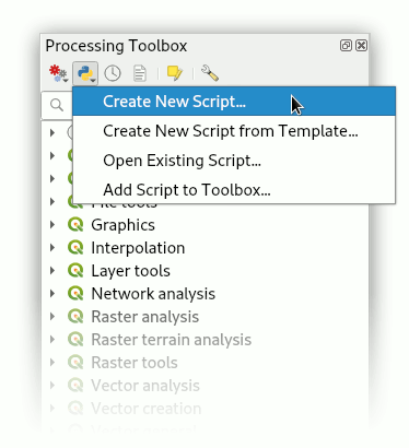
Copy-and-paste the template code from before into the editor window that opens and immediately make the following changes:
- Rename the class from
RENAME_THISto a meaningful name. (line 12) Python code style guidelines recommend a CapWords style, i.e. each word in the class name starts with an uppercase letter. The class name should refer to the function of the class. We are building a tool, let’s revisit how we refer to physical-world tools: a good example is Screwdriver – it’s a tool to drive (insert) a screw (into some material). Were it a software tool, a good class name would be
ScrewDriver. Our tool rasterises species range maps, let’s call itSpeciesRangeMapsRasteriser.
- Rename the class from
- Change the display name of our tool. (line 21)
The names of most of the algorithms in the processing toolbox consist of a verb and an object (e.g. “Create spatial index”). Let’s stick with this concept and call our tool “Rasterise species range maps”.
- Save these changes.
Choose a filename representing the tool (e.g. SpeciesRangeMapsRasteriser.py, and save it in the default directory.
You can now already run the script (press the play button in the editor window) and find it in the toolbox (in scripts). Since we did not define any parameters or algorithms, the script does nothing, though.
Define script parameters
The class method initAlgorithm() defines general characteristics of a toolbox algorithm, such as which parameters are accepted. It is being run whenever QGIS updates the list of algorithms installed, for instance when QGIS starts or when a script is saved in the editor.
Use the self.addParameter() method to define parameters, self.addOutput() to define outputs of the algorithm.
Our script has three parameters:
An input vector layer
The name of the field containing the species name
A directory to save the output to (for practical reasons, in this example, this is an input parameter, it can also be implemented as an output)
The parameters are objects (instances) of one of the classes QgsProcessingParameter*, documented in qgis.org/pyqgis/3.4/core/Processing/, and have to be imported from qgis.core at the beginning of the script. We will use QgsProcessingParameterVectorLayer, QgsProcessingParameterField and QgsProcessingParameterFolderDestination. We can add them to the existing import statement:
from qgis.core import (
     QgsProcessing,
     QgsProcessingAlgorithm,
     QgsProcessingParameterField,
     QgsProcessingParameterFolderDestination,
     QgsProcessingParameterVectorLayer
 )
For each of the parameters, we call self.addParameter() inside initAlgorithm():
def initAlgorithm(self, config=None):
    self.addParameter(
        QgsProcessingParameterVectorLayer(
            name="SpeciesRangePolygons",
            description="Species range polygons",
            types=[QgsProcessing.SourceType.TypeVectorPolygon]
        )
    )
    self.addParameter(
        QgsProcessingParameterField(
            name="SpeciesAttribute",
            description="Species attribute",
            parentLayerParameterName="SpeciesRangePolygons",
            type=QgsProcessingParameterField.String
        )
    )
    self.addParameter(
        QgsProcessingParameterFolderDestination(
            name="OutputFolder",
            description="Output folder"
        )
    )
As you can see, the QgsProcessingParameter* classes need to be initialised with arguments. All of them share name and description, which will be used for labelling the controls in the user interface. We can specify the geometry type of the vector layer, and define which layer the field should be chosen from, and which type of field is allowed.
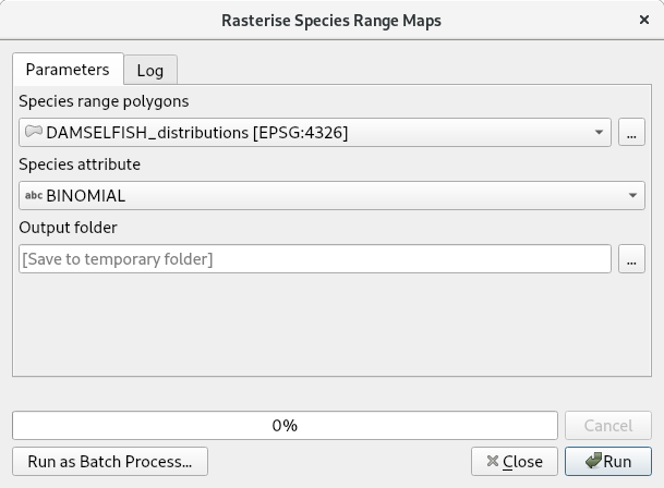
Save the script and try to run it: You’ll see the user interface asking for input.
Program the algorithm
All of the following will be added to the processAlgorithm() method. The function receives a few arguments, one of them, parameters is a dict containing the parameters defined in the user interface.
As a very first step, we make sure the output directory exists:
# 0)
# create destination directory
os.makedirs(
    parameters["OutputFolder"],
    exist_ok=True
)
We use the function makedirs of the os module, which we thus have to add to the import statements in the beginning of the file.
Add a new field and update its value
Next, we need to add a new field with a user-defined name. We use a hard-coded field name of presence and fill it with the hard-coded value of 1 for all features of the layer. This value will later be used to fill the raster grid values.
For this step, we use the field calculator algorithm of the processing toolbox. To find its scripting name (id), search for it, then display its help text on the Python console (not the editor window):
# search for “buffer” algorithms:
In [3]: searchTerm = "calculator"
In [4]: print([a.id() for a in QgsApplication.processingRegistry().algorithms() if searchTerm in a.id()])
Out[4]: ['qgis:advancedpythonfieldcalculator', 'qgis:fieldcalculator', 'qgis:rastercalculator']
In [5]: processing.algorithmHelp
Out[5]: Field calculator (qgis:fieldcalculator)

This algorithm computes a new vector layer with the same features of the input layer, but with an additional attribute. The values of this new attribute are computed from each feature using a mathematical formula, based on the properties and attributes of the feature.


----------------
Input parameters
----------------

INPUT:  <QgsProcessingParameterFeatureSource>
        Input layer

FIELD_NAME:  <QgsProcessingParameterString>
        Result field name

FIELD_TYPE:  <QgsProcessingParameterEnum>
        Field type
                0 - Float
                1 - Integer
                2 - String
                3 - Date

FIELD_LENGTH:  <QgsProcessingParameterNumber>
        Field length

FIELD_PRECISION:  <QgsProcessingParameterNumber>
        Field precision

NEW_FIELD:  <QgsProcessingParameterBoolean>
        Create new field

FORMULA:  <QgsProcessingParameterExpression>
        Formula

OUTPUT:  <QgsProcessingParameterFeatureSink>
        Calculated

----------------
Outputs
----------------

OUTPUT:  <QgsProcessingOutputVectorLayer>
        Calculated
We use processing.run() to run the algorithm, and have to supply the algorithm’s id and input parameters in a dictionary. run() returns a dictionary with all output values, amongst them the output layer. Add the following section of code to the processAlgorithm() method (in the editor window).
# 1)
# add a new integer field `presence` with value 1
# (input for rasterising later on)
algorithmOutput = processing.run(
    "qgis:fieldcalculator",
    {
        "INPUT": parameters["SpeciesRangePolygons"],
        "NEW_FIELD": True,
        "FIELD_NAME": "presence",
        "FIELD_TYPE": 1,
        "FORMULA": "1",
        "OUTPUT": "memory:speciesRangePolygonsWithPresenceValue"
    },
    context=context,
    feedback=feedback
)
speciesRangePolygonsWithPresenceValue = algorithmOutput["OUTPUT"]
Find unique species
As we wanted to save individual species into separate raster files, we need to determine the unique species in our attribute table. For this, we will use the layer’s uniqueValues() function, which requires a field’s index instead of its name. This function is somewhat equivalent to Geopandas unique().
# 2)
# Find all distinct species names
fields = parameters["SpeciesRangePolygons"].fields()
fieldIndex = fields.indexFromName(parameters["SpeciesAttribute"])
speciesNames = \
    parameters["SpeciesRangePolygons"].uniqueValues(fieldIndex)
Select by attribute and rasterise
Now, for each species we run three algorithms: we use select by attribute (qgis:selectbyattribute) to save the features belonging to the current species into a new layer. Because the rasterize algorithm does not understand the default in-memory vector file format, we write the vector data to an intermediate file and then convert the vector data into a raster file using the rasterize (vector to raster) tool (gdal:rasterize). Before that, we have to define an output file name for our raster. At the end of each loop, we delete the intermediate shapefile.
# 3)
# Loop over all species
for speciesName in speciesNames:
    if speciesName is not None:

        # 3a)
        # define output file name:
        outputFile = os.path.join(
            parameters["OutputFolder"],
            speciesName.replace(" ", "_")
        )

        # 3b)
        # select all features with current `speciesName`
        algorithmOutput = processing.run(
            "qgis:selectbyattribute",
            {
                "INPUT": speciesRangePolygonsWithPresenceValue,
                "FIELD": parameters["SpeciesAttribute"],
                "OPERATOR": 0,
                "VALUE": speciesName,
                "METHOD": 0
            },
            context=context,
            feedback=feedback                )
        singleSpeciesRangePolygons = algorithmOutput["OUTPUT"]

        # 3c)
        # save intermediate vector file
        algorithmOutput = processing.run(
            "native:saveselectedfeatures",
            {
                "INPUT": singleSpeciesRangePolygons,
                "OUTPUT": outputFile + ".shp"
            },
            context=context,
            feedback=feedback
        )
        singleSpeciesRangePolygons = algorithmOutput["OUTPUT"]

        # 3d)
        # rasterise the vector layer
        algorithmOutput = processing.run(
            "gdal:rasterize",
            {
                "INPUT": singleSpeciesRangePolygons,

                "FIELD": "presence",

                "UNITS": 0,
                "WIDTH": 2000,
                "HEIGHT": 1000,
                "EXTENT": "-180, 180, -90, 90",

                "RTYPE": 0,
                "OUTPUT": outputFile + ".tif"
            },
            context=context,
            feedback=feedback
        )

        # 3f)
        # delete intermediate vector file
        os.remove(outputFile + ".shp")
Return the result
processAlgorithm() is expected to return a dictionary with computed values or layers. Since our algorithm does not have an output (except the files saved into the specified directory) we simply return an empty dictionary:
return {}
Run the script
To run the script, find it from the toolbox, select DAMSELFISH Distributions as the input layer, BINOMIAL as the species attribute, and specify an output directory. Then click Run.
The full script
#!/bin/env python

import os
import os.path
import processing
import string

from qgis.core import (
    QgsProcessing,
    QgsProcessingAlgorithm,
    QgsProcessingParameterField,
    QgsProcessingParameterFolderDestination,
    QgsProcessingParameterVectorLayer
)

class RasteriseSpeciesRangeMaps(QgsProcessingAlgorithm):

    def __init__(self):
        super().__init__()

    def createInstance(self):
        return type(self)()

    def displayName(self):
        return "Rasterise species range maps"

    def name(self):
        name = "".join([
            character for character in self.displayName().lower()
            if character in string.ascii_letters
        ])
        return name

    def initAlgorithm(self, config=None):
        self.addParameter(
            QgsProcessingParameterVectorLayer(
                name="SpeciesRangePolygons",
                description="Species range polygons",
                types=[QgsProcessing.SourceType.TypeVectorPolygon]
            )
        )
        self.addParameter(
            QgsProcessingParameterField(
                name="SpeciesAttribute",
                description="Species attribute",
                parentLayerParameterName="SpeciesRangePolygons",
                type=QgsProcessingParameterField.String
            )
        )
        self.addParameter(
            QgsProcessingParameterFolderDestination(
                name="OutputFolder",
                description="Output folder"
            )
        )

    def processAlgorithm(self, parameters, context, feedback):
        # 0)
        # create destination directory
        os.makedirs(
            parameters["OutputFolder"],
            exist_ok=True
        )

        # 1)
        # add a new integer field `presence` with value 1
        # (input for rasterising later on)
        algorithmOutput = processing.run(
            "qgis:fieldcalculator",
            {
                "INPUT": parameters["SpeciesRangePolygons"],
                "NEW_FIELD": True,
                "FIELD_NAME": "presence",
                "FIELD_TYPE": 1,
                "FORMULA": "1",
                "OUTPUT": "memory:speciesRangePolygonsWithPresenceValue"
            },
            context=context,
            feedback=feedback
        )
        speciesRangePolygonsWithPresenceValue = algorithmOutput["OUTPUT"]

        # 2)
        # Find all distinct species names
        fields = parameters["SpeciesRangePolygons"].fields()
        fieldIndex = fields.indexFromName(parameters["SpeciesAttribute"])
        speciesNames = \
            parameters["SpeciesRangePolygons"].uniqueValues(fieldIndex)

        # 3)
        # Loop over all species
        for speciesName in speciesNames:
            if speciesName is not None:

                # 3a)
                # define output file name:
                outputFile = os.path.join(
                    parameters["OutputFolder"],
                    speciesName.replace(" ", "_")
                )

                # 3b)
                # select all features with current `speciesName`
                algorithmOutput = processing.run(
                    "qgis:selectbyattribute",
                    {
                        "INPUT": speciesRangePolygonsWithPresenceValue,
                        "FIELD": parameters["SpeciesAttribute"],
                        "OPERATOR": 0,
                        "VALUE": speciesName,
                        "METHOD": 0
                    },
                    context=context,
                    feedback=feedback                )
                singleSpeciesRangePolygons = algorithmOutput["OUTPUT"]

                # 3c)
                # save intermediate vector file
                algorithmOutput = processing.run(
                    "native:saveselectedfeatures",
                    {
                        "INPUT": singleSpeciesRangePolygons,
                        "OUTPUT": outputFile + ".shp"
                    },
                    context=context,
                    feedback=feedback
                )
                singleSpeciesRangePolygons = algorithmOutput["OUTPUT"]

                # 3d)
                # rasterise the vector layer
                algorithmOutput = processing.run(
                    "gdal:rasterize",
                    {
                        "INPUT": singleSpeciesRangePolygons,

                        "FIELD": "presence",

                        "UNITS": 0,
                        "WIDTH": 2000,
                        "HEIGHT": 1000,
                        "EXTENT": "-180, 180, -90, 90",

                        "RTYPE": 0,
                        "OUTPUT": outputFile + ".tif"
                    },
                    context=context,
                    feedback=feedback
                )

                # 3f)
                # delete intermediate vector file
                os.remove(outputFile + ".shp")

        return {}
- 1
“online” in the sense of context-sensitive help from within the command line interface. Not necessarily refering to the internet in any way.
- 2
This is a minimal template, sufficient for this exercise. You can also use the built-in template by choosing Create new script from template …. The resulting skeleton script is more complex, but also more comprehensive.