Spatial join
Spatial join is yet another classic GIS problem. Getting attributes from one layer and transferring them into another layer based on their spatial relationship is something you most likely need to do on a regular basis.
In the previous section we learned how to perform a Point in Polygon query.
We could now apply those techniques and create our own function to perform a spatial join between two layers based on their
spatial relationship. We could, for example, join the attributes of a polygon layer into a point layer where each point would get the
attributes of a polygon that contains the point.
Luckily, spatial join is already implemented in Geopandas
, thus we do not need to create it ourselves. There are three possible types of
join that can be applied in spatial join that are determined with op -parameter in the gpd.sjoin() -function:
"intersects""within""contains"
Sounds familiar? Yep, all of those spatial relationships were discussed in the Point in Polygon lesson, thus you should know how they work.
Let’s perform a spatial join between these two layers:
Addresses: the address-point Shapefile that we created trough geocoding
Population grid: a Polygon layer that is a 250m x 250m grid showing the amount of people living in the Helsinki Region.
The population grid a dataset is produced by the Helsinki Region Environmental Services Authority (HSY) (see this page to access data from different years).
For this lesson we will use the population grid for year 2017, which can be dowloaded as a shapefile from this link in the Helsinki Region Infroshare (HRI) open data portal
Download and clean the data
Execute the following steps in a terminal window
Navigate to the data folder
$ cd data
Download the population grid using wget:
$ wget "https://www.hsy.fi/sites/AvoinData/AvoinData/SYT/Tietoyhteistyoyksikko/Shape%20(Esri)/V%C3%A4est%C3%B6tietoruudukko/Vaestotietoruudukko_2017_SHP.zip"
Unzip the file in Terminal into a folder called Pop17 (using -d flag)
$ unzip Vaestotietoruudukko_2017_SHP.zip -d Pop17
You should now have a folder /data/Pop17 containing the population grid shapefile.
Let’s read the data into memory and see what we have.
import geopandas as gpd

# Filepath
fp = "data/Pop17/Vaestoruudukko_2017.shp"

# Read the data
pop = gpd.read_file(fp)

# See the first rows
pop.head()
| INDEX | ASUKKAITA | ASVALJYYS | IKA0_9 | IKA10_19 | IKA20_29 | IKA30_39 | IKA40_49 | IKA50_59 | IKA60_69 | IKA70_79 | IKA_YLI80 | geometry | |
|---|---|---|---|---|---|---|---|---|---|---|---|---|---|
| 0 | 688 | 9 | 28.0 | 99 | 99 | 99 | 99 | 99 | 99 | 99 | 99 | 99 | POLYGON Z ((25472499.99532626 6689749.00506918... |
| 1 | 710 | 8 | 44.0 | 99 | 99 | 99 | 99 | 99 | 99 | 99 | 99 | 99 | POLYGON Z ((25472499.99532626 6684249.00413040... |
| 2 | 711 | 5 | 90.0 | 99 | 99 | 99 | 99 | 99 | 99 | 99 | 99 | 99 | POLYGON Z ((25472499.99532626 6683999.00499700... |
| 3 | 715 | 12 | 37.0 | 99 | 99 | 99 | 99 | 99 | 99 | 99 | 99 | 99 | POLYGON Z ((25472499.99532626 6682998.99846143... |
| 4 | 848 | 6 | 44.0 | 99 | 99 | 99 | 99 | 99 | 99 | 99 | 99 | 99 | POLYGON Z ((25472749.99291839 6690249.00333598... |
Okey so we have multiple columns in the dataset but the most important
one here is the column ASUKKAITA (“population” in Finnish) that
tells the amount of inhabitants living under that polygon.
Let’s change the name of that columns into
pop17so that it is more intuitive. Changing column names is easy in Pandas / Geopandas using a function calledrename()where we pass a dictionary to a parametercolumns={'oldname': 'newname'}.
# Change the name of a column
pop = pop.rename(columns={'ASUKKAITA': 'pop17'})

# See the column names and confirm that we now have a column called 'pop17'
pop.columns
Index(['INDEX', 'pop17', 'ASVALJYYS', 'IKA0_9', 'IKA10_19', 'IKA20_29',
       'IKA30_39', 'IKA40_49', 'IKA50_59', 'IKA60_69', 'IKA70_79', 'IKA_YLI80',
       'geometry'],
      dtype='object')
Let’s also get rid of all unnecessary columns by selecting only columns that we need i.e.
pop17andgeometry
# Columns that will be sected
selected_cols = ['pop17', 'geometry']

# Select those columns
pop = pop[selected_cols]

# Let's see the last 2 rows
pop.head()
| pop17 | geometry | |
|---|---|---|
| 0 | 9 | POLYGON Z ((25472499.99532626 6689749.00506918... |
| 1 | 8 | POLYGON Z ((25472499.99532626 6684249.00413040... |
| 2 | 5 | POLYGON Z ((25472499.99532626 6683999.00499700... |
| 3 | 12 | POLYGON Z ((25472499.99532626 6682998.99846143... |
| 4 | 6 | POLYGON Z ((25472749.99291839 6690249.00333598... |
Now we have cleaned the data and have only those columns that we need for our analysis.
Join the layers
Now we are ready to perform the spatial join between the two layers that
we have. The aim here is to get information about how many people live
in a polygon that contains an individual address-point . Thus, we want
to join attributes from the population layer we just modified into the
addresses point layer addresses.shp that we created trough gecoding in the previous section.
Read the addresses layer into memory
# Addresses filpath
addr_fp = r"data/addresses.shp"

# Read data
addresses = gpd.read_file(addr_fp)

# Check the head of the file
addresses.head()
| address | id | addr | geometry | |
|---|---|---|---|---|
| 0 | Ruoholahti, 14, Itämerenkatu, Ruoholahti, Läns... | 1000 | Itämerenkatu 14, 00101 Helsinki, Finland | POINT (24.9155624 60.1632015) |
| 1 | Kamppi, 1, Kampinkuja, Kamppi, Eteläinen suurp... | 1001 | Kampinkuja 1, 00100 Helsinki, Finland | POINT (24.9316914 60.1690222) |
| 2 | Bangkok9, 8, Kaivokatu, Keskusta, Kluuvi, Etel... | 1002 | Kaivokatu 8, 00101 Helsinki, Finland | POINT (24.9416849 60.1699637) |
| 3 | 1, Hermannin rantatie, Hermanninmäki, Hermanni... | 1003 | Hermannin rantatie 1, 00580 Helsinki, Finland | POINT (24.9655355 60.2008878) |
| 4 | Hesburger, 9, Tyynenmerenkatu, Jätkäsaari, Län... | 1005 | Tyynenmerenkatu 9, 00220 Helsinki, Finland | POINT (24.9216003 60.1566475) |
In order to do a spatial join, the layers need to be in the same projection
# Are the layers in the same projection?
addresses.crs == pop.crs
False
Let’s re-project addresses to the projection of the population layer:
addresses = addresses.to_crs(pop.crs)
Let’s make sure that the coordinate reference system of the layers are identical
# Check the crs of address points
print(addresses.crs)

# Check the crs of population layer
print(pop.crs)

# Do they match now?
addresses.crs == pop.crs
{'proj': 'tmerc', 'lat_0': 0, 'lon_0': 25, 'k': 1, 'x_0': 25500000, 'y_0': 0, 'ellps': 'GRS80', 'units': 'm', 'no_defs': True}
{'proj': 'tmerc', 'lat_0': 0, 'lon_0': 25, 'k': 1, 'x_0': 25500000, 'y_0': 0, 'ellps': 'GRS80', 'units': 'm', 'no_defs': True}
True
Now they should be identical. Thus, we can be sure that when doing spatial queries between layers the locations match and we get the right results e.g. from the spatial join that we are conducting here.
Let’s now join the attributes from
popGeoDataFrame intoaddressesGeoDataFrame by usinggpd.sjoin()-function
# Make a spatial join
join = gpd.sjoin(addresses, pop, how="inner", op="within")

# Let's check the result
join.head()
| address | id | addr | geometry | index_right | pop17 | |
|---|---|---|---|---|---|---|
| 0 | Ruoholahti, 14, Itämerenkatu, Ruoholahti, Läns... | 1000 | Itämerenkatu 14, 00101 Helsinki, Finland | POINT (25495311.60802662 6672258.694634228) | 3238 | 501 |
| 1 | Kamppi, 1, Kampinkuja, Kamppi, Eteläinen suurp... | 1001 | Kampinkuja 1, 00100 Helsinki, Finland | POINT (25496207.84010911 6672906.172794735) | 3350 | 190 |
| 2 | Bangkok9, 8, Kaivokatu, Keskusta, Kluuvi, Etel... | 1002 | Kaivokatu 8, 00101 Helsinki, Finland | POINT (25496762.72293893 6673010.538330208) | 3474 | 37 |
| 10 | Rautatientori, Keskusta, Kluuvi, Eteläinen suu... | 1011 | Rautatientori 1, 00100 Helsinki, Finland | POINT (25496896.60078502 6673159.446016792) | 3474 | 37 |
| 3 | 1, Hermannin rantatie, Hermanninmäki, Hermanni... | 1003 | Hermannin rantatie 1, 00580 Helsinki, Finland | POINT (25498088.55200266 6676455.030033929) | 3711 | 133 |
Awesome! Now we have performed a successful spatial join where we got
two new columns into our join GeoDataFrame, i.e. index_right
that tells the index of the matching polygon in the population grid and
pop17 which is the population in the cell where the address-point is
located.
Let’s save this layer into a new Shapefile
# Output path
outfp = r"data/addresses_pop17_epsg3979.shp"

# Save to disk
join.to_file(outfp)
Do the results make sense? Let’s evaluate this a bit by plotting the points where color intensity indicates the population numbers.
Plot the points and use the
pop17column to indicate the color.cmap-parameter tells to use a sequential colormap for the values,markersizeadjusts the size of a point,schemeparameter can be used to adjust the classification method based on pysal, andlegendtells that we want to have a legend.
import matplotlib.pyplot as plt

# Plot the points with population info
join.plot(column='pop17', cmap="Reds", markersize=7, scheme='quantiles', legend=True);

# Add title
plt.title("Amount of inhabitants living close the the point");

# Remove white space around the figure
plt.tight_layout()
/opt/conda/lib/python3.6/site-packages/scipy/stats/stats.py:1713: FutureWarning: Using a non-tuple sequence for multidimensional indexing is deprecated; use `arr[tuple(seq)]` instead of `arr[seq]`. In the future this will be interpreted as an array index, `arr[np.array(seq)]`, which will result either in an error or a different result.
  return np.add.reduce(sorted[indexer] * weights, axis=axis) / sumval
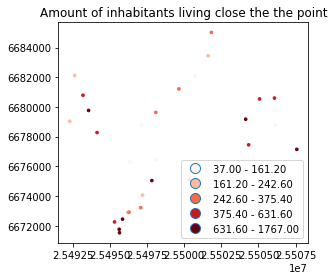
By knowing approximately how population is distributed in Helsinki, it seems that the results do make sense as the points with highest population are located in the south where the city center of Helsinki is.