Geopandas: an introduction

In this section, we will cover the basics of geopandas, a Python library to interact with geospatial vector data.

Geopandas provides an easy-to-use interface to vector data sets. It combines the capabilities of pandas, the data analysis package we got to know in the Geo-Python course, with the geometry handling functionality of shapely, the geo-spatial file format support of fiona and the map projection libraries of pyproj.

The main data structures in geopandas are GeoDataFrames and GeoSeries. They extend the functionality of pandas.DataFrames and pandas.Series. This means that we can use all our pandas skills also when we work with geopandas!.

Tip

If you feel like you need to refresh your memory about pandas, head back to lesson 5 and lesson 6 of Geo-Python.

There is one key difference between pandas’s data frames and geopandas’ GeoDataFrames: a GeoDataFrame contains an additional column for geometries. By default, the name of this column is geometry, and it is a GeoSeries that contains the geometries (points, lines, polygons, …) as shapely.geometry objects.

	GROUP	CLASS	geometry
0	64	32421	POLYGON ((379394.248 6689991.936, 379389 ...
1	64	32421	POLYGON ((378980.811 6689359.377, 378983 ...
2	64	32421	POLYGON ((378804.766 6689256.471, 378817 ...
3	64	32421	POLYGON ((379229.695 6685025.111, 379233 ...
4	64	32421	POLYGON ((379825.199 6685096.247, 379829 ...

---

Input data: Finnish topographic database

In this lesson, we will work with the National Land Survey of Finland (NLS)/Maanmittauslaitos (MML) topographic database.

• The data set is licensed under the NLS’ open data licence (CC BY 4.0).

• The structure of the data is described in a separate Excel file.

• Further information about file naming is available at fairdata.fi (this link relates to the 2018 issue of the topographic database, but is still valid).

For this lesson, we have acquired a subset of the topographic database as shapefiles from the Helsinki Region in Finland via the CSC’s Paituli download portal. You can find the files in data/finland_topographic_database/.

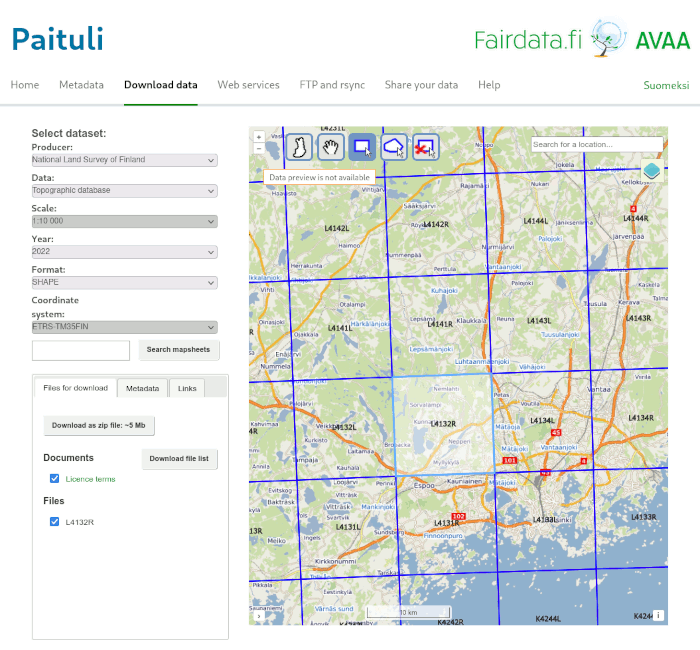
The Paituli spatial download service offers data from a long list of national institutes and agencies.

---

Read and explore geo-spatial data sets

Before we attempt to load any files, let’s not forget to defining a constant that points to our data directory:

import pathlib 
NOTEBOOK_PATH = pathlib.Path().resolve()
DATA_DIRECTORY = NOTEBOOK_PATH / "data"

In this lesson, we will focus on terrain objects (Feature group: “Terrain/1” in the topographic database). The Terrain/1 feature group contains several feature classes.

Our aim in this lesson is to save all the Terrain/1 feature classes into separate files.

Terrain/1 features in the Topographic Database:

feature class	Name of feature	Feature group
32421	Motor traffic area	Terrain/1
32200	Cemetery	Terrain/1
34300	Sand	Terrain/1
34100	Rock - area	Terrain/1
34700	Rocky area	Terrain/1
32500	Quarry	Terrain/1
32112	Mineral resources extraction area, fine-grained material	Terrain/1
32111	Mineral resources extraction area, coarse-grained material	Terrain/1
32611	Field	Terrain/1
32612	Garden	Terrain/1
32800	Meadow	Terrain/1
32900	Park	Terrain/1
35300	Paludified land	Terrain/1
35412	Bog, easy to traverse forested	Terrain/1
35411	Open bog, easy to traverse treeless	Terrain/1
35421	Open fen, difficult to traverse treeless	Terrain/1
33000	Earth fill	Terrain/1
33100	Sports and recreation area	Terrain/1
36200	Lake water	Terrain/1
36313	Watercourse area	Terrain/1

Search for files using a pattern

A pathlib.Path (such as DATA_DIRECTORY) has a handy method to list all files in a directory (or subdirectories) that match a pattern: glob(). To list all shapefiles in our topographic database directory, we can use the following expression:

(DATA_DIRECTORY / "finland_topographic_database").glob("*.shp")

In the search pattern, ? represents any one single character, * multiple (or none, or one) characters, and ** multiple characters that can include subdirectories.

Did you notice the parentheses in the code example above? They work just like they would in a mathematical expression: first, the expression inside the parentheses is evaluated, only then, the code outside.

If you take a quick look at the data directory using a file browser, you will notice that the topographic database consists of many smaller files. Their names follow a strictly defined convention, according to this file naming convention, all files that we interested in (Terrain/1 and polygons) start with a letter m and end with a p.

We can use the glob() pattern search functionality to find those files:

TOPOGRAPHIC_DATABASE_DIRECTORY = DATA_DIRECTORY / "finland_topographic_database"

TOPOGRAPHIC_DATABASE_DIRECTORY

PosixPath('/home/docs/checkouts/readthedocs.org/user_builds/autogis-site/checkouts/latest/docs/lessons/lesson-2/data/finland_topographic_database')

list(TOPOGRAPHIC_DATABASE_DIRECTORY.glob("m*p.shp"))

[PosixPath('/home/docs/checkouts/readthedocs.org/user_builds/autogis-site/checkouts/latest/docs/lessons/lesson-2/data/finland_topographic_database/m_L4132R_p.shp')]

(Note that glob() returns an iterator, but, for now, we quickly convert it to a list)

It seems our input data set has only one file that matches our search pattern. We can save its filename into a new variable, choosing the first item of the list (index 0):

input_filename = list(TOPOGRAPHIC_DATABASE_DIRECTORY.glob("m*p.shp"))[0] 

Now, it’s finally time to open the file and look at its contents:

import geopandas
data = geopandas.read_file(input_filename)

First, check the data type of the read data set:

type(data)

geopandas.geodataframe.GeoDataFrame

Everything went fine, and we have a geopandas.GeoDataFrame. Let’s also explore the data: (1) print the first few rows, and (2) list the columns.

data.head()

	TEKSTI	RYHMA	LUOKKA	TASTAR	KORTAR	KORARV	KULKUTAPA	KOHDEOSO	AINLAHDE	SYNTYHETKI	...	TOLEFT	FROMRIGHT	TORIGHT	TIENIM2	TIENIM3	TIENIM4	TIENIM5	KUNTA_NRO	KUNTA	geometry
0	None	64	32421	5000	0	0.0	0	1812247077	1	20180125	...	0	0	0	None	None	None	None	0	None	POLYGON ((379394.248 6689991.936, 379389.790 6...
1	None	64	32421	5000	0	0.0	0	1718796908	1	20180120	...	0	0	0	None	None	None	None	0	None	POLYGON ((378980.811 6689359.377, 378983.401 6...
2	None	64	32421	20000	0	0.0	0	411167695	1	20180120	...	0	0	0	None	None	None	None	0	None	POLYGON ((378804.766 6689256.471, 378817.107 6...
3	None	64	32421	20000	0	0.0	0	411173768	1	20180120	...	0	0	0	None	None	None	None	0	None	POLYGON ((379229.695 6685025.111, 379233.366 6...
4	None	64	32421	20000	0	0.0	0	411173698	1	20180120	...	0	0	0	None	None	None	None	0	None	POLYGON ((379825.199 6685096.247, 379829.651 6...

5 rows × 39 columns

data.columns

Index(['TEKSTI', 'RYHMA', 'LUOKKA', 'TASTAR', 'KORTAR', 'KORARV', 'KULKUTAPA',
       'KOHDEOSO', 'AINLAHDE', 'SYNTYHETKI', 'KUOLHETKI', 'KARTOGLK',
       'ALUEJAKOON', 'VERSUH', 'SUUNTA', 'SIIRT_DX', 'SIIRT_DY', 'KORKEUS',
       'PYSYVAID', 'ATTR3', 'TIENUM', 'OSANUM', 'TIEOSA', 'PAALLY', 'YKSSUU',
       'VAPKOR', 'VALMAS', 'PITUUS', 'FROMLEFT', 'TOLEFT', 'FROMRIGHT',
       'TORIGHT', 'TIENIM2', 'TIENIM3', 'TIENIM4', 'TIENIM5', 'KUNTA_NRO',
       'KUNTA', 'geometry'],
      dtype='object')

Oh boy! This data set has many columns, and all of the column names are in Finnish.

Let’s select a few useful ones and also translate their names to English. We’ll keep ’RYHMA’ and ’LUOKKA’ (‘group’ and ‘class’, respectively), and, of course, the geometry column.

data = data[["RYHMA", "LUOKKA", "geometry"]]

Renaming a column in (geo)pandas works by passing a dictionary to DataFrame.rename(). In this dictionary, the keys are the old names, the values the new ones:

data = data.rename(
    columns={
        "RYHMA": "GROUP",
        "LUOKKA": "CLASS"
    }
)

How does the data set look now?

data.head()

	GROUP	CLASS	geometry
0	64	32421	POLYGON ((379394.248 6689991.936, 379389.790 6...
1	64	32421	POLYGON ((378980.811 6689359.377, 378983.401 6...
2	64	32421	POLYGON ((378804.766 6689256.471, 378817.107 6...
3	64	32421	POLYGON ((379229.695 6685025.111, 379233.366 6...
4	64	32421	POLYGON ((379825.199 6685096.247, 379829.651 6...

Check your understanding:

Use your pandas skills on this geopandas data set to figure out the following information:

• How many rows does the data set have?

• How many unique classes?

• … and how many unique groups?

---

Explore the data set in a map:

As geographers, we love maps. But beyond that, it’s always a good idea to explore a new data set also in a map. To create a simple map of a geopandas.GeoDataFrame, simply use its plot() method. It works similar to pandas (see Lesson 7 of the Geo-Python course, but draws a map based on the geometries of the data set instead of a chart.

data.plot()

<AxesSubplot: >

Voilá! It is indeed this easy to produce a map out of an geospatial data set. Geopandas automatically positions your map in a way that it covers the whole extent of your data.

Note

If you live in the Helsinki region, you might recognise some of the shapes in the map ;)

Geometries in geopandas

Geopandas takes advantage of shapely’s geometry objects. Geometries are stored in a column called geometry.

Let’s print the first 5 rows of the column geometry:

data.geometry.head()

0    POLYGON ((379394.248 6689991.936, 379389.790 6...
1    POLYGON ((378980.811 6689359.377, 378983.401 6...
2    POLYGON ((378804.766 6689256.471, 378817.107 6...
3    POLYGON ((379229.695 6685025.111, 379233.366 6...
4    POLYGON ((379825.199 6685096.247, 379829.651 6...
Name: geometry, dtype: geometry

Lo and behold, the geometry column contains familiar-looking values: Well-Known Text (WKT) strings. Don’t be fooled, they are, in fact, shapely.geometry objects (you might remember from last week’s lesson) that, when print()ed or type-cast into a str, are represented as a WKT string).

Since the geometries in a GeoDataFrame are stored as shapely objects, we can use shapely methods to handle geometries in geopandas.

Let’s take a closer look at (one of) the polygon geometries in the terrain data set, and try to use some of the shapely functionality we are already familiar with. For the sake of clarity, first, we’ll work with the geometry of the very first record, only:

# The value of the column `geometry` in row 0:
data.at[0, "geometry"]

# Print information about the area 
print(f"Area: {round(data.at[0, 'geometry'].area)} m².")

Area: 76 m².

Area measurement unit

Here, we know the coordinate reference system (CRS) of the input data set. The CRS also defines the unit of measurement (in our case, metres). That’s why we can print the computed area including an area measurement unit (square metres).

Let’s do the same for multiple rows, and explore different options of how to. First, use the reliable and tried iterrows() pattern we learned in lesson 6 of the Geo-Python course.

# Iterate over the first 5 rows of the data set
for index, row in data[:5].iterrows():
    polygon_area = row["geometry"].area
    print(f"The polygon in row {index} has a surface area of {polygon_area:0.1f} m².")

The polygon in row 0 has a surface area of 76.0 m².
The polygon in row 1 has a surface area of 2652.1 m².
The polygon in row 2 has a surface area of 3185.6 m².
The polygon in row 3 has a surface area of 13075.2 m².
The polygon in row 4 has a surface area of 3980.7 m².

As you see, all pandas functions, such as the iterrows() method, are available in geopandas without the need to call pandas separately. Geopandas builds on top of pandas, and it inherits most of its functionality.

Of course the iterrows() pattern is not the most convenient and efficient way to calculate the area of many rows. Both GeoSeries (geometry columns) and GeoDataFrames have an area property:

# the `area` property of a `GeoDataFrame`
data.area

0          76.027392
1        2652.054186
2        3185.649995
3       13075.165279
4        3980.682621
            ...     
4299     2651.800270
4300      376.503380
4301      413.942555
4302     3487.927677
4303     1278.963199
Length: 4304, dtype: float64

# the `area property of a `GeoSeries`
data["geometry"].area

0          76.027392
1        2652.054186
2        3185.649995
3       13075.165279
4        3980.682621
            ...     
4299     2651.800270
4300      376.503380
4301      413.942555
4302     3487.927677
4303     1278.963199
Length: 4304, dtype: float64

It’s straight-forward to create a new column holding the area:

data["area"] = data.area
data

	GROUP	CLASS	geometry	area
0	64	32421	POLYGON ((379394.248 6689991.936, 379389.790 6...	76.027392
1	64	32421	POLYGON ((378980.811 6689359.377, 378983.401 6...	2652.054186
2	64	32421	POLYGON ((378804.766 6689256.471, 378817.107 6...	3185.649995
3	64	32421	POLYGON ((379229.695 6685025.111, 379233.366 6...	13075.165279
4	64	32421	POLYGON ((379825.199 6685096.247, 379829.651 6...	3980.682621
...	...	...	...	...
4299	64	36313	POLYGON ((375668.607 6682942.062, 375671.489 6...	2651.800270
4300	64	36313	POLYGON ((368411.063 6679328.990, 368411.424 6...	376.503380
4301	64	36313	POLYGON ((368054.608 6679164.737, 368059.602 6...	413.942555
4302	64	36313	POLYGON ((368096.331 6678000.000, 368090.276 6...	3487.927677
4303	64	36313	POLYGON ((368000.666 6678460.142, 368000.000 6...	1278.963199

4304 rows × 4 columns

Descriptive statistics

Do you remember how to calculate the minimum, maximum, sum, mean, and standard deviation of a pandas column? (Lesson 5 of Geo-Python) What are these values for the area column of the data set?

Write a subset of data to a file

In the previous section, we learnt how to write an entire GeoDataFrame to a file. We can also write a filtered subset of a data set to a new file, e.g., to help with processing complex data sets.

First, isolate the lakes in the input data set (class number 36200, see table above):

lakes = data[data.CLASS == 36200]

Then, plot the data subset to visually check whether it looks correct:

lakes.plot()

<AxesSubplot: >

And finally, write the filtered data to a Shapefile:

lakes.to_file(DATA_DIRECTORY / "finland_topographic_database" / "lakes.shp")

Check the Vector Data I/O section to see which data formats geopandas can write to.

Grouping data

A particularly useful method of (geo)pandas’ data frames is their grouping function: groupby() can split data into groups based on some criteria, apply a function individually to each of the groups, and combine results of such an operation into a common data structure.

We have used this function earlier: in Geo-Python, lesson 6.

We can use grouping here to split our input data set into subsets that relate to each of the CLASSes of terrain cover, then save a separate file for each class.

Let’s start this by, again, taking a look at how the data set actually looks like:

data.head()

	GROUP	CLASS	geometry	area
0	64	32421	POLYGON ((379394.248 6689991.936, 379389.790 6...	76.027392
1	64	32421	POLYGON ((378980.811 6689359.377, 378983.401 6...	2652.054186
2	64	32421	POLYGON ((378804.766 6689256.471, 378817.107 6...	3185.649995
3	64	32421	POLYGON ((379229.695 6685025.111, 379233.366 6...	13075.165279
4	64	32421	POLYGON ((379825.199 6685096.247, 379829.651 6...	3980.682621

Remember: the CLASS column contains information about a polygon’s land use type. Use the pandas.Series.unique() method to list all values that occur:

data["CLASS"].unique()

array([32421, 32200, 34300, 34100, 34700, 32417, 32500, 32112, 32111,
       32611, 32612, 32800, 32900, 35300, 35412, 35411, 35421, 33000,
       33100, 36200, 36313])

To group data, use the data frame’s groupby() method, supply a column name as a parameter:

grouped_data = data.groupby("CLASS")
grouped_data

<pandas.core.groupby.generic.DataFrameGroupBy object at 0x7f7c915b4280>

So, grouped_data is a DataFrameGroupBy object. Inside a GroupBy object, its property groups is a dictionary that works as a lookup table: it records which rows belong to which group. The keys of the dictionary are the unique values of the grouping column:

grouped_data.groups

{32111: [3116], 32112: [3115], 32200: [103, 104], 32417: [3112], 32421: [0, 1, 2, 3, 4, 5, 6, 7, 8, 9, 10, 11, 12, 13, 14, 15, 16, 17, 18, 19, 20, 21, 22, 23, 24, 25, 26, 27, 28, 29, 30, 31, 32, 33, 34, 35, 36, 37, 38, 39, 40, 41, 42, 43, 44, 45, 46, 47, 48, 49, 50, 51, 52, 53, 54, 55, 56, 57, 58, 59, 60, 61, 62, 63, 64, 65, 66, 67, 68, 69, 70, 71, 72, 73, 74, 75, 76, 77, 78, 79, 80, 81, 82, 83, 84, 85, 86, 87, 88, 89, 90, 91, 92, 93, 94, 95, 96, 97, 98, 99, ...], 32500: [3113, 3114], 32611: [3117, 3118, 3119, 3120, 3121, 3122, 3123, 3124, 3125, 3126, 3127, 3128, 3129, 3130, 3131, 3132, 3133, 3135, 3136, 3137, 3138, 3139, 3140, 3141, 3142, 3143, 3144, 3145, 3146, 3147, 3148, 3149, 3150, 3151, 3152, 3153, 3154, 3155, 3156, 3157, 3158, 3159, 3160, 3161, 3162, 3163, 3164, 3165, 3166, 3167, 3168, 3169, 3170, 3171, 3172, 3173, 3174, 3175, 3176, 3177, 3178, 3179, 3180, 3181, 3182, 3183, 3184, 3185, 3186, 3187, 3188, 3189, 3190, 3191, 3192, 3193, 3194, 3195, 3196, 3197, 3198, 3199, 3200, 3201, 3202, 3203, 3204, 3205, 3206, 3207, 3208, 3209, 3210, 3211, 3212, 3213, 3214, 3215, 3216, 3217, ...], 32612: [3134, 3224, 3242, 3245, 3265, 3266, 3283, 3326, 3327, 3378, 3380], 32800: [3389, 3390, 3391, 3392, 3393, 3394, 3395, 3396, 3397, 3398, 3399, 3400, 3401, 3402, 3403, 3404, 3405, 3406, 3407, 3408, 3409, 3410, 3411, 3412, 3413, 3414, 3415, 3416, 3417, 3418, 3419, 3420, 3421, 3422, 3423, 3424, 3425, 3426, 3427, 3428, 3429, 3430, 3431, 3432, 3433, 3434, 3435, 3436, 3437, 3438, 3439, 3440, 3441, 3442, 3443, 3444, 3445, 3446, 3447, 3448, 3449, 3450, 3451, 3452, 3453, 3454, 3455, 3456, 3457, 3458, 3459, 3460, 3461, 3462, 3463, 3464, 3465, 3466, 3467, 3468, 3469], 32900: [3470, 3471, 3472, 3473, 3474, 3475, 3476, 3477, 3478, 3479, 3480, 3481, 3482, 3483, 3484, 3485, 3486, 3487, 3488, 3489, 3490, 3491, 3492, 3493, 3494, 3495], 33000: [4118, 4119, 4120, 4121, 4122], 33100: [4123, 4124, 4125, 4126, 4127, 4128, 4129, 4130, 4131, 4132, 4133, 4134, 4135, 4136, 4137, 4138, 4139, 4140, 4141, 4142, 4143, 4144, 4145, 4146, 4147, 4148, 4149, 4150, 4151, 4152, 4153, 4154, 4155, 4156, 4157, 4158, 4159, 4160, 4161, 4162, 4163, 4164, 4165, 4166, 4167, 4168, 4169, 4170, 4171, 4172, 4173, 4174, 4175, 4176, 4177, 4178, 4179, 4180, 4181, 4182, 4183, 4184, 4185, 4186, 4187, 4188, 4189, 4190, 4191, 4192, 4193, 4194, 4195, 4196, 4197, 4198, 4199, 4200, 4201, 4202, 4203, 4204, 4205, 4206, 4207, 4208, 4209, 4210, 4211, 4212, 4213, 4214, 4215, 4216, 4217, 4218, 4219, 4220, 4221, 4222, ...], 34100: [106, 107, 108, 109, 110, 111, 112, 113, 114, 115, 116, 117, 118, 119, 120, 121, 122, 123, 124, 125, 126, 127, 128, 129, 130, 131, 132, 133, 134, 135, 136, 137, 138, 139, 140, 141, 142, 143, 144, 145, 146, 147, 148, 149, 150, 151, 152, 153, 154, 155, 156, 157, 158, 159, 160, 161, 162, 163, 164, 165, 166, 167, 168, 169, 170, 171, 172, 173, 174, 175, 176, 177, 178, 179, 180, 181, 182, 183, 184, 185, 186, 187, 188, 189, 190, 191, 192, 193, 194, 195, 196, 197, 198, 199, 200, 201, 202, 203, 204, 205, ...], 34300: [105], 34700: [3109, 3110, 3111], 35300: [3496, 3497, 3498, 3499, 3500, 3501, 3502, 3503, 3504, 3505, 3506, 3507, 3508, 3509, 3510, 3511, 3512, 3513, 3514, 3515, 3516, 3517, 3518, 3519, 3520, 3521, 3522, 3523, 3524, 3525, 3526, 3527, 3528, 3529, 3530, 3531, 3532, 3533, 3534, 3535, 3536, 3537, 3538, 3539, 3540, 3541, 3542, 3543, 3544, 3545, 3546, 3547, 3548, 3549, 3550, 3551, 3552, 3553, 3554, 3555, 3556, 3557, 3558, 3559, 3560, 3561, 3562, 3563, 3564, 3565, 3566, 3567, 3568, 3569, 3570, 3571, 3572, 3573, 3574, 3575, 3576, 3577, 3578, 3579, 3580, 3581, 3582, 3583, 3584, 3585, 3586, 3587, 3588, 3589, 3590, 3591, 3592, 3593, 3594, 3595, ...], 35411: [3637, 3638, 3643, 3652, 3717, 3720, 3733, 3734, 3735, 3742, 3753, 3754, 3779, 3802, 3820, 3822, 3844, 3925, 3950, 4002, 4003, 4005, 4053, 4055, 4056, 4062, 4070, 4072, 4087, 4095, 4103, 4105, 4106, 4112], 35412: [3630, 3631, 3632, 3633, 3634, 3635, 3636, 3639, 3640, 3641, 3642, 3644, 3645, 3646, 3647, 3648, 3649, 3650, 3653, 3654, 3655, 3656, 3657, 3658, 3659, 3660, 3661, 3662, 3663, 3664, 3665, 3666, 3667, 3668, 3669, 3671, 3672, 3673, 3674, 3675, 3676, 3677, 3678, 3679, 3680, 3681, 3682, 3683, 3684, 3685, 3686, 3687, 3688, 3689, 3690, 3691, 3692, 3693, 3694, 3695, 3696, 3697, 3698, 3699, 3700, 3701, 3702, 3704, 3705, 3706, 3707, 3708, 3709, 3710, 3711, 3712, 3713, 3714, 3715, 3716, 3718, 3719, 3721, 3722, 3723, 3724, 3725, 3726, 3727, 3728, 3729, 3730, 3731, 3732, 3736, 3737, 3738, 3739, 3740, 3741, ...], 35421: [3651, 3670, 3703, 3755, 3758], 36200: [4240, 4241, 4242, 4243, 4244, 4245, 4246, 4247, 4248, 4249, 4250, 4251, 4252, 4253, 4254, 4255, 4256, 4257, 4258, 4259, 4260, 4261, 4262, 4263, 4264, 4265, 4266, 4267, 4268, 4269, 4270, 4271, 4272, 4273, 4274, 4275, 4276, 4277, 4278, 4279, 4280, 4281, 4282, 4283, 4284, 4285, 4286, 4287, 4288, 4289, 4290, 4291, 4292, 4293, 4294, 4295], 36313: [4296, 4297, 4298, 4299, 4300, 4301, 4302, 4303]}

However, one can also simply iterate over the entire GroupBy object. Let’s count how many rows of data each group has:

for key, group in grouped_data:
    print(f"Terrain class {key} has {len(group)} rows.")

Terrain class 32111 has 1 rows.
Terrain class 32112 has 1 rows.
Terrain class 32200 has 2 rows.
Terrain class 32417 has 1 rows.
Terrain class 32421 has 103 rows.
Terrain class 32500 has 2 rows.
Terrain class 32611 has 261 rows.
Terrain class 32612 has 11 rows.
Terrain class 32800 has 81 rows.
Terrain class 32900 has 26 rows.
Terrain class 33000 has 5 rows.
Terrain class 33100 has 117 rows.
Terrain class 34100 has 3003 rows.
Terrain class 34300 has 1 rows.
Terrain class 34700 has 3 rows.
Terrain class 35300 has 134 rows.
Terrain class 35411 has 34 rows.
Terrain class 35412 has 449 rows.
Terrain class 35421 has 5 rows.
Terrain class 36200 has 56 rows.
Terrain class 36313 has 8 rows.

There are, for instance, 56 lake polygons (class 36200) in the input data set.

To obtain all rows that belong to one particular group, use the get_group() method, which returns a brand-new GeoDataFrame:

lakes = grouped_data.get_group(36200)
type(lakes)

geopandas.geodataframe.GeoDataFrame

Caution

The index in the new data frame stays the same as in the ungrouped input data set. This can be helpful, for instance, when you want to join the grouped data back to the original input data.

Write grouped data to separate files

Now we have all the necessary tools in hand to split the input data into separate data sets for each terrain class, and write the individual subsets to new, separate, files. In fact, the code looks almost too simple, doesn’t it?

# Iterate over the input data, grouped by CLASS
for key, group in data.groupby("CLASS"):
    # save the group to a new shapefile
    group.to_file(TOPOGRAPHIC_DATABASE_DIRECTORY / f"terrain_{key}.shp")

File name

We used a pathlib.Path combined with an f-string to generate the new output file’s path and name. Check this week’s section Managing file paths, and Geo-Python lesson 2 to revisit how they work.

Extra: save summary statistics to CSV spreadsheet

Whenever the results of an operation on a GeoDataFrame do not include a geometry, the output data frame will automatically become a ‘plain’ pandas.DataFrame, and can be saved to the standard table formats.

One interesting application of this is to save basic descriptive statistics of a geospatial data set into a CSV table. For instance, we might want to know the area each terrain class covers.

Again, we start by grouping the input data by terrain classes, and then compute the sum of each classes’ area. This can be condensed into one line of code:

area_information = data.groupby("CLASS").area.sum()
area_information

CLASS
32111    1.833747e+03
32112    2.148168e+03
32200    1.057368e+05
32417    1.026678e+02
32421    6.792797e+05
32500    1.097467e+05
32611    1.314807e+07
32612    1.073431e+05
32800    1.407231e+06
32900    6.158391e+05
33000    6.594647e+05
33100    3.769076e+06
34100    1.236289e+07
34300    1.627079e+03
34700    2.785751e+03
35300    1.382940e+06
35411    3.928004e+05
35412    4.708321e+06
35421    6.786374e+04
36200    9.986966e+06
36313    4.346029e+04
Name: area, dtype: float64

We can then save the resulting table into a CSV file using the standard pandas approach we learned about in Geo-Python lesson 5.

area_information.to_csv(TOPOGRAPHIC_DATABASE_DIRECTORY / "area_by_terrain_class.csv")