Spatial join

Spatial joins are operations that combine data from two or more spatial data sets based on their geometric relationship. In the previous sections, we got to know two specific cases of spatial joins: Point-in-polygon queries and intersects-queries. However, there is more to using the geometric relationship between features and between entire layers.

Spatial join operations require two input parameters: the predicament, i.e., the geometric condition that needs to be met between two geometries, and the join-type: whether only rows with matching geometries are kept, or all of one input table’s rows, or all records.

Geopandas (using shapely to implement geometric relationships) supports a standard set of geometric predicates, that is similar to most GIS analysis tools and applications:

• intersects

• contains

• within

• touches

• crosses

• overlaps

Geometric predicaments are expressed as verbs, so they have an intuitive meaning. See the shapely user manual for a detailed description of each geometric predicate.

Binary geometric predicates

Shapely supports more binary geometric predicates than geopandas implements for spatial joins. What are they? Can they be expressed by combining the implemented ones?

In terms of the join-type, geopandas implements three different options:

• left: keep all records of the left data frame, fill with empty values if no match, keep left geometry column

• right: keep all records of the left data frame, fill with empty values if no match, keep right geometry column

• inner: keep only records of matching records, keep left geometry column

Tip

The PyGIS book has a great overview of spatial predicaments and join-types with explanatory drawings.

---

Load input data

As a practical example, let’s find the population density at each of the addresses from earlier in this lesson, by combining the data set with data from a population grid.

The population grid data is available from HSY, the Helsinki Region Environmental Services, for instance via their WFS endpoint.

import pathlib 
NOTEBOOK_PATH = pathlib.Path().resolve()
DATA_DIRECTORY = NOTEBOOK_PATH / "data"

import geopandas

addresses = geopandas.read_file(DATA_DIRECTORY / "addresses.gpkg")

population_grid = geopandas.read_file(
    (
        "https://kartta.hsy.fi/geoserver/wfs"
        "?service=wfs"
        "&version=2.0.0"
        "&request=GetFeature"
        "&typeName=asuminen_ja_maankaytto:Vaestotietoruudukko_2020"
        "&srsName=EPSG:3879"
    ),
)
population_grid.crs = "EPSG:3879"  # for WFS data, the CRS needs to be specified manually

Concatenating long strings

In the WFS address above, we split a long string across multiple lines. Strings between parentheses are automatically concatenated (joint together), even without any operator (e.g., +).

For the sake of clarity, the example has an additional set of parentheses, but already the parentheses of the method call would suffice.

---

population_grid.head()

	asukkaita	geometry
0	5	POLYGON ((25472499.995 6689749.005, 25472499.9...
1	7	POLYGON ((25472499.995 6685998.998, 25472499.9...
2	8	POLYGON ((25472499.995 6684249.004, 25472499.9...
3	7	POLYGON ((25472499.995 6683999.005, 25472499.9...
4	11	POLYGON ((25472499.995 6682998.998, 25472499.9...

The population grid has many columns, and all of its column names are in Finnish. Let’s drop (delete) all of the columns except the population total, and rename the remaining to English:

population_grid = population_grid[["asukkaita", "geometry"]]
population_grid = population_grid.rename(columns={"asukkaita": "population"})

Finally, calculate the population density by dividing the number of inhabitants of each grid cell by its area in km²:

population_grid["population_density"] = (
    population_grid["population"]
    / (population_grid.area / 1_000_000)
)
population_grid.head()

	population	geometry	population_density
0	5	POLYGON ((25472499.995 6689749.005, 25472499.9...	80.001048
1	7	POLYGON ((25472499.995 6685998.998, 25472499.9...	112.001467
2	8	POLYGON ((25472499.995 6684249.004, 25472499.9...	128.001677
3	7	POLYGON ((25472499.995 6683999.005, 25472499.9...	112.001467
4	11	POLYGON ((25472499.995 6682998.998, 25472499.9...	176.002305

Coding style: big numbers, operators in multi-line expressions

If you need to use very large numbers, such as, in the above example, the 1 million to convert m² to km², you can use underscore characters (_) as thousands separators. The Python interpreter will treat a sequence of numbers interleaved with underscores as a regular numeric value. You can use the same syntax to group numbers by a different logic, for instance, to group hexadecimal or binary values into groups of four.

In case an expression, such as, e.g., a mathematical formula, spreads across multiple lines, it is considered good coding style to place an operator at the beginning of a new line, rather than let it trail in the previous line. This is considered more readable, as explained in the PEP-8 styling guidelines

---

Join input layers

Now we are ready to perform the spatial join between the two layers. Remember: the aim is to find the population density around each of the address points. We want to attach population density information from the population_grid polygon layer to the addresses point layer, depending on whether the point is within the polygon. During this operation, we want to retain the geometries of the point layer.

Before we can go ahead with the join operation, we have to make sure the two layers are in the same cartographic reference system:

assert addresses.crs == population_grid.crs, "CRS are not identical"

---------------------------------------------------------------------------
AssertionError                            Traceback (most recent call last)
Cell In [6], line 1
----> 1 assert addresses.crs == population_grid.crs, "CRS are not identical"

AssertionError: CRS are not identical

They do not share the same CRS, let’s reproject one of them:

population_grid = population_grid.to_crs(addresses.crs)

Now we are ready to carry out the actual spatial join using the geopandas.GeoDataFrame.sjoin() method. Remember, we want to use a within geometric predicate and retain the point layer’s geometries (in the example below the left data frame).

addresses_with_population_data = addresses.sjoin(
    population_grid,
    how="left",
    predicate="within"
)
addresses_with_population_data.head()

	address	geometry	index_right	population	population_density
0	Ruoholahti, 14, Itämerenkatu, Salmisaari, Ruoh...	POINT (24.91556 60.16320)	3262.0	505.0	8080.105832
1	Kamppi, 1, Kampinkuja, Kamppi, Eteläinen suurp...	POINT (24.93166 60.16905)	3381.0	172.0	2752.036046
2	Kauppakeskus Citycenter, 8, Kaivokatu, Keskust...	POINT (24.94179 60.16989)	3504.0	43.0	688.009011
3	Hermannin rantatie, Verkkosaari, Kalasatama, S...	POINT (24.97846 60.19206)	NaN	NaN	NaN
4	9, Tyynenmerenkatu, Jätkäsaari, Länsisatama, E...	POINT (24.92151 60.15662)	3310.0	1402.0	22431.538035

That looks great! We now have an address data set with population density information attached to it.

---

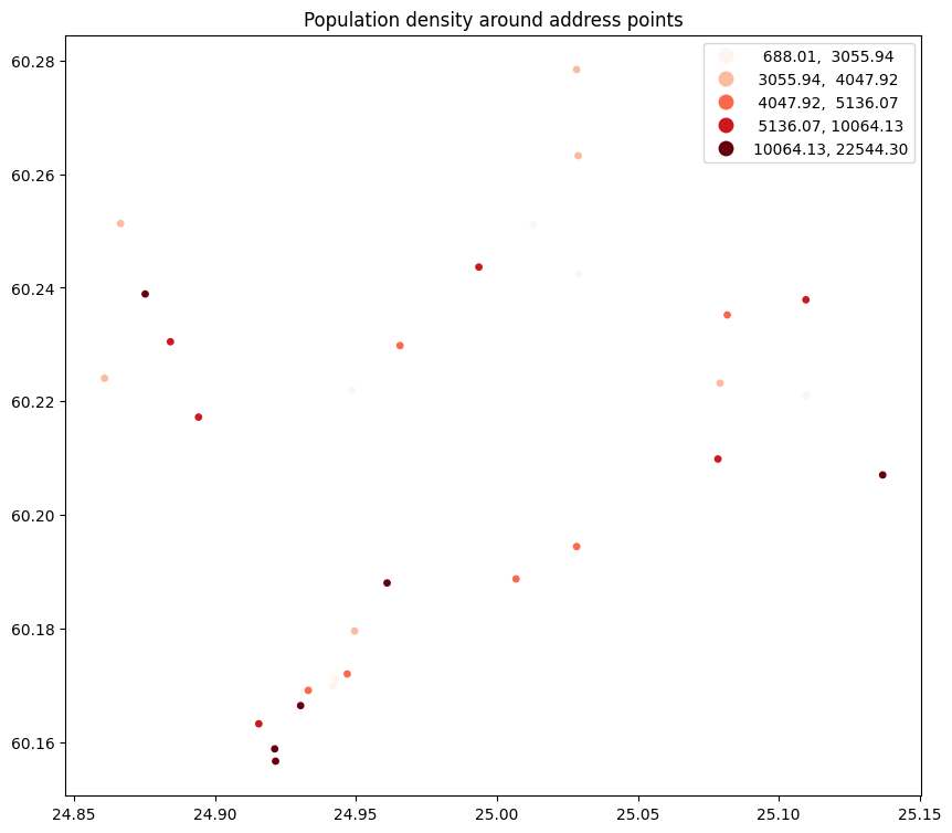
As a final task, let’s look at how to plot data using a graduated cartographic visualisation scheme.

The geopandas.GeoDataFrame.plot() method can vary the map colours depending on a column’s values by passing its name as a named argument column. On top of that, the method accepts many arguments to influence the style of the map. Among them are scheme and cmap that define the categorisation scheme, and the colour map used. Many more arguments are passed through to matplotlib, such as markersize to set the size of point symbols, and facecolor to set the colour of polygon areas. To draw a legend, set legend to True, to set the size of the figure, pass a tuple (with values in inch) as figsize.

ax = addresses_with_population_data.plot(
    figsize=(10, 10),
    column="population_density",
    cmap="Reds",
    scheme="quantiles",
    markersize=15,
    legend=True
)
ax.set_title("Population density around address points")

Text(0.5, 1.0, 'Population density around address points')

---

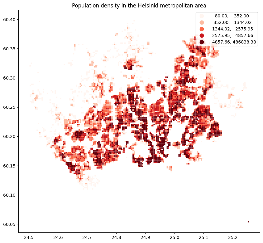
We can apply the same arguments to plot a population density map using the entire population_grid data set:

ax = population_grid.plot(
    figsize=(10, 10),
    column="population_density",
    cmap="Reds",
    scheme="quantiles",
    legend=True
)
ax.set_title("Population density in the Helsinki metropolitan area")

Text(0.5, 1.0, 'Population density in the Helsinki metropolitan area')

---

Finally, remember to save the output data frame to a file. We can append it to the existing GeoPackage by specifying a new layer name:

addresses_with_population_data.to_file(
    DATA_DIRECTORY / "addresses.gpkg",
    layer="addresses_with_population_data"
)