Overlay analysis

Overlay analyses are GIS operations in which two or more vector layers are combined to produce new geometries. Typical overlay operations include union, intersection, and difference - named after the result of the combination of two layers.

Spatial overlay with two input vector layers (rectangle, circle). The resulting vector layer is displayed in green. Source: QGIS documentation

In this tutorial, we will carry out an overlay analysis to select those polygon cells of a grid dataset that lie within the city limits of Helsinki. For this exercise, we use two input data sets: a grid of statistical polygons with the travel time to the Helsinki railway station, covering the entire metropolitan area (helsinki_region_travel_times_to_railway_station.gpkg) and a polygon data set (with one feature) of the area the municipality of Helsinki covers (helsinki_municipality.gpkg). Both files are in logically named subfolders of the DATA_DIRECTORY.

import pathlib 
NOTEBOOK_PATH = pathlib.Path().resolve()
DATA_DIRECTORY = NOTEBOOK_PATH / "data"

import geopandas

grid = geopandas.read_file(
    DATA_DIRECTORY
    / "helsinki_region_travel_times_to_railway_station"
    / "helsinki_region_travel_times_to_railway_station.gpkg"
)

helsinki = geopandas.read_file(
    DATA_DIRECTORY / "helsinki_municipality" / "helsinki_municipality.gpkg"
)

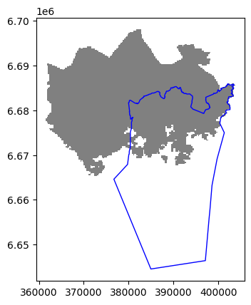
Let’s do a quick overlay visualization of the two layers:

# Plot the layers
ax = grid.plot(facecolor="gray")
helsinki.plot(ax=ax, facecolor="None", edgecolor="blue")

<AxesSubplot: >

Here the grey area is the Travel Time Matrix - a data set that contains 13231 grid squares (13231 rows of data) that covers the Helsinki region, and the blue area represents the municipality of Helsinki. Our goal is to conduct an overlay analysis and select the geometries from the grid polygon layer that intersect with the Helsinki municipality polygon.

When conducting overlay analysis, it is important to first check that the CRS of the layers match. The overlay visualization indicates that everything should be ok (the layers are plotted nicely on top of each other). However, let’s still check if the crs match using Python:

# Check the crs of the municipality polygon
print(helsinki.crs)

epsg:3067

# Ensure that the CRS matches, if not raise an AssertionError
assert helsinki.crs == grid.crs, "CRS differs between layers!"

Indeed, they do. We are now ready to conduct an overlay analysis between these layers.

We will create a new layer based on grid polygons that intersect with our Helsinki layer. We can use a method overlay() of a GeoDataFrame to conduct the overlay analysis that takes as an input 1) second GeoDataFrame, and 2) parameter how that can be used to control how the overlay analysis is conducted (possible values are 'intersection', 'union', 'symmetric_difference', 'difference', and 'identity'):

intersection = grid.overlay(helsinki, how="intersection")

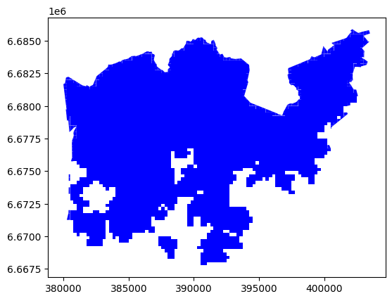
Let’s plot our data and see what we have:

intersection.plot(color="b")

<AxesSubplot: >

As a result, we now have only those grid cells that intersect with the Helsinki borders. If you look closely, you can also observe that the grid cells are clipped based on the boundary.

• Whatabout the data attributes? Let’s see what we have:

intersection.head()

	car_m_d	car_m_t	car_r_d	car_r_t	from_id	pt_m_d	pt_m_t	pt_m_tt	pt_r_d	pt_r_t	pt_r_tt	to_id	walk_d	walk_t	GML_ID	NAMEFIN	NAMESWE	NATCODE	geometry
0	29476	41	29483	46	5876274	29990	76	95	24984	77	99	5975375	25532	365	27517366	Helsinki	Helsingfors	091	POLYGON ((402024.224 6685750.000, 402003.328 6...
1	29456	41	29462	46	5876275	29866	74	95	24860	75	93	5975375	25408	363	27517366	Helsinki	Helsingfors	091	POLYGON ((402250.000 6685750.000, 402250.000 6...
2	36772	50	36778	56	5876278	33541	116	137	44265	130	146	5975375	31110	444	27517366	Helsinki	Helsingfors	091	POLYGON ((403148.515 6685750.000, 403243.781 6...
3	36898	49	36904	56	5876279	33720	119	141	44444	132	155	5975375	31289	447	27517366	Helsinki	Helsingfors	091	POLYGON ((403250.000 6685750.000, 403250.000 6...
4	29411	40	29418	44	5878128	29944	75	95	24938	76	99	5975375	25486	364	27517366	Helsinki	Helsingfors	091	POLYGON ((401900.425 6685500.000, 402000.000 6...

As we can see, due to the overlay analysis, the dataset contains the attributes from both input layers.

Let’s save our result grid as a GeoPackage.

intersection.to_file(
    DATA_DIRECTORY / "intersection.gpkg",
    layer="travel_time_matrix_helsinki_region"
)

There are many more examples for different types of overlay analysis in Geopandas documentation where you can go and learn more.