Aggregating data

Data aggregation refers to a process where we combine data into groups. When doing spatial data aggregation, we merge the geometries together into coarser units (based on some attribute), and can also calculate summary statistics for these combined geometries from the original, more detailed values. For example, suppose that we are interested in studying continents, but we only have country-level data like the country dataset. If we aggregate the data by continent, we would convert the country-level data into a continent-level dataset.

In this tutorial, we will aggregate our travel time data by car travel times (column car_r_t), i.e. the grid cells that have the same travel time to Railway Station will be merged together.

Let’s start with loading intersection.gpkg, the output file of the previous section:

import pathlib 
NOTEBOOK_PATH = pathlib.Path().resolve()
DATA_DIRECTORY = NOTEBOOK_PATH / "data"

import geopandas
intersection = geopandas.read_file(DATA_DIRECTORY / "intersection.gpkg")

For doing the aggregation we will use a method called dissolve() that takes as input the column that will be used for conducting the aggregation:

# Conduct the aggregation
dissolved = intersection.dissolve(by="car_r_t")

# What did we get
dissolved.head()

	geometry	car_m_d	car_m_t	car_r_d	from_id	pt_m_d	pt_m_t	pt_m_tt	pt_r_d	pt_r_t	pt_r_tt	to_id	walk_d	walk_t	GML_ID	NAMEFIN	NAMESWE	NATCODE
car_r_t
-1	MULTIPOLYGON (((384750.000 6670000.000, 384500...	-1	-1	-1	5913094	-1	-1	-1	-1	-1	-1	-1	-1	-1	27517366	Helsinki	Helsingfors	091
0	POLYGON ((385750.000 6672000.000, 385750.000 6...	0	0	0	5975375	0	0	0	0	0	0	5975375	0	0	27517366	Helsinki	Helsingfors	091
7	POLYGON ((386250.000 6671750.000, 386000.000 6...	1051	7	1051	5973739	617	5	6	617	5	6	5975375	448	6	27517366	Helsinki	Helsingfors	091
8	MULTIPOLYGON (((386000.000 6671500.000, 385750...	1286	8	1286	5973736	706	10	10	706	10	10	5975375	706	10	27517366	Helsinki	Helsingfors	091
9	MULTIPOLYGON (((385000.000 6671250.000, 385000...	1871	9	1871	5970457	1384	11	13	1394	11	12	5975375	1249	18	27517366	Helsinki	Helsingfors	091

Let’s compare the number of cells in the layers before and after the aggregation:

print(f"Rows in original intersection GeoDataFrame: {len(intersection)}")
print(f"Rows in dissolved layer: {len(dissolved)}")

Rows in original intersection GeoDataFrame: 3826
Rows in dissolved layer: 51

Indeed the number of rows in our data has decreased and the Polygons were merged together.

What actually happened here? Let’s take a closer look.

Let’s see what columns we have now in our GeoDataFrame:

dissolved.columns

Index(['geometry', 'car_m_d', 'car_m_t', 'car_r_d', 'from_id', 'pt_m_d',
       'pt_m_t', 'pt_m_tt', 'pt_r_d', 'pt_r_t', 'pt_r_tt', 'to_id', 'walk_d',
       'walk_t', 'GML_ID', 'NAMEFIN', 'NAMESWE', 'NATCODE'],
      dtype='object')

As we can see, the column that we used for conducting the aggregation (car_r_t) can not be found from the columns list anymore. What happened to it?

Let’s take a look at the indices of our GeoDataFrame:

dissolved.index

Int64Index([-1,  0,  7,  8,  9, 10, 11, 12, 13, 14, 15, 16, 17, 18, 19, 20, 21,
            22, 23, 24, 25, 26, 27, 28, 29, 30, 31, 32, 33, 34, 35, 36, 37, 38,
            39, 40, 41, 42, 43, 44, 45, 46, 47, 48, 49, 50, 51, 52, 53, 54,
            56],
           dtype='int64', name='car_r_t')

Aha! Well now we understand where our column went. It is now used as index in our dissolved GeoDataFrame.

Now, we can for example select only such geometries from the layer that are for example exactly 15 minutes away from the Helsinki Railway Station:

# Select only geometries that are within 15 minutes away
dissolved.loc[15]

/home/docs/checkouts/readthedocs.org/user_builds/autogis-site/envs/latest/lib/python3.10/site-packages/pandas/core/dtypes/inference.py:387: ShapelyDeprecationWarning: Iteration over multi-part geometries is deprecated and will be removed in Shapely 2.0. Use the `geoms` property to access the constituent parts of a multi-part geometry.
  iter(obj)  # Can iterate over it.
/home/docs/checkouts/readthedocs.org/user_builds/autogis-site/envs/latest/lib/python3.10/site-packages/pandas/core/dtypes/inference.py:388: ShapelyDeprecationWarning: __len__ for multi-part geometries is deprecated and will be removed in Shapely 2.0. Check the length of the `geoms` property instead to get the  number of parts of a multi-part geometry.
  len(obj)  # Has a length associated with it.
/home/docs/checkouts/readthedocs.org/user_builds/autogis-site/envs/latest/lib/python3.10/site-packages/pandas/io/formats/printing.py:117: ShapelyDeprecationWarning: Iteration over multi-part geometries is deprecated and will be removed in Shapely 2.0. Use the `geoms` property to access the constituent parts of a multi-part geometry.
  s = iter(seq)
/home/docs/checkouts/readthedocs.org/user_builds/autogis-site/envs/latest/lib/python3.10/site-packages/pandas/io/formats/printing.py:121: ShapelyDeprecationWarning: __len__ for multi-part geometries is deprecated and will be removed in Shapely 2.0. Check the length of the `geoms` property instead to get the  number of parts of a multi-part geometry.
  for i in range(min(nitems, len(seq)))
/home/docs/checkouts/readthedocs.org/user_builds/autogis-site/envs/latest/lib/python3.10/site-packages/pandas/io/formats/printing.py:125: ShapelyDeprecationWarning: __len__ for multi-part geometries is deprecated and will be removed in Shapely 2.0. Check the length of the `geoms` property instead to get the  number of parts of a multi-part geometry.
  if nitems < len(seq):

geometry    (POLYGON ((384000.00013620744 6670750.00004266...
car_m_d                                                  7458
car_m_t                                                    13
car_r_d                                                  7458
from_id                                               5934913
pt_m_d                                                   6858
pt_m_t                                                     26
pt_m_tt                                                    30
pt_r_d                                                   6858
pt_r_t                                                     27
pt_r_tt                                                    32
to_id                                                 5975375
walk_d                                                   6757
walk_t                                                     97
GML_ID                                               27517366
NAMEFIN                                              Helsinki
NAMESWE                                           Helsingfors
NATCODE                                                   091
Name: 15, dtype: object

# See the data type
type(dissolved.loc[15])

pandas.core.series.Series

As we can see, as a result, we have now a Pandas Series object containing basically one row from our original aggregated GeoDataFrame.

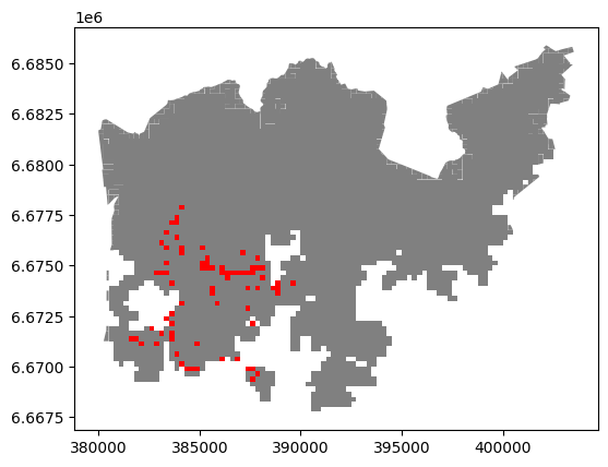
Let’s also visualize those 15 minute grid cells.

First, we need to convert the selected row back to a GeoDataFrame:

# Create a GeoDataFrame
selection = geopandas.GeoDataFrame([dissolved.loc[15]], crs=dissolved.crs)

Plot the selection on top of the entire grid:

# Plot all the grid cells, and the grid cells that are 15 minutes
# away from the Railway Station
ax = dissolved.plot(facecolor="gray")
selection.plot(ax=ax, facecolor="red")

<AxesSubplot: >

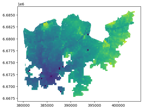
Another way to visualize the travel times in the entire GeoDataFrame is to plot using one specific column. In order to use our car_r_t column, which is now the index of the GeoDataFrame, we need to reset the index:

dissolved = dissolved.reset_index()
dissolved.head()

	car_r_t	geometry	car_m_d	car_m_t	car_r_d	from_id	pt_m_d	pt_m_t	pt_m_tt	pt_r_d	pt_r_t	pt_r_tt	to_id	walk_d	walk_t	GML_ID	NAMEFIN	NAMESWE	NATCODE
0	-1	MULTIPOLYGON (((384750.000 6670000.000, 384500...	-1	-1	-1	5913094	-1	-1	-1	-1	-1	-1	-1	-1	-1	27517366	Helsinki	Helsingfors	091
1	0	POLYGON ((385750.000 6672000.000, 385750.000 6...	0	0	0	5975375	0	0	0	0	0	0	5975375	0	0	27517366	Helsinki	Helsingfors	091
2	7	POLYGON ((386250.000 6671750.000, 386000.000 6...	1051	7	1051	5973739	617	5	6	617	5	6	5975375	448	6	27517366	Helsinki	Helsingfors	091
3	8	MULTIPOLYGON (((386000.000 6671500.000, 385750...	1286	8	1286	5973736	706	10	10	706	10	10	5975375	706	10	27517366	Helsinki	Helsingfors	091
4	9	MULTIPOLYGON (((385000.000 6671250.000, 385000...	1871	9	1871	5970457	1384	11	13	1394	11	12	5975375	1249	18	27517366	Helsinki	Helsingfors	091

As we can see, we now have our car_r_t as a column again, and can then plot the GeoDataFrame passing this column using the column parameter:

dissolved.plot(column="car_r_t")

<AxesSubplot: >