Map projections

A coordinate reference systems (CRS) is a crucial piece of metadata for any geospatial data set. Without a CRS, the geometries would simply be a collection of coordinates in an arbitrary space. Only the CRS allows GIS software, including the Python packages we use in this course, to relate these coordinates to a place on Earth (or other approximately spherical objects or planets).

Often conflated with coordinate reference systems, and definitely closely related, are map projections. Map projections, also called projected coordinate systems, are mathematical models that allow us to transfer coordinates on the surface of our three-dimensional Earth into coordinates in a planar surface, such as a flat, two-dimensional map. In contrast to projected coordinate systems, geographic coordinate systems simply directly use latitude and longitude, i.e. the degrees along the horizontal and vertical great circles of a sphere approximating the Earth, as the x and y coordinates in a planar map. Finally, there are both projected and geographic coordinate systems that make use of more complex ellipsoids than a simple sphere to better approximate the ‘potato-shaped’ reality of our planet. The full CRS information needed to accurately relate geospatial information to a place on Earth includes both (projected/geographic) coordinate system and ellipsoid.

The CRS in different spatial datasets differ fairly often, as different coordinate systems are optimised for certain regions and purposes. No coordinate system can be perfectly accurate around the globe, and the transformation from three- to two-dimensional coordinates can not be accurate in angles, distances, and areas simultaneously.

Consequently, it is a common GIS task to transform (or reproject) a data set from one references system into another, for instance, to make two layers interoperatable. Comparing two data sets that have different CRS would inevitably produce wrong results; for example, finding points contained within a polygon cannot work, if the the points have geographic coordinates (in degrees), and the polygon is in the national Finnish reference system (in meters).

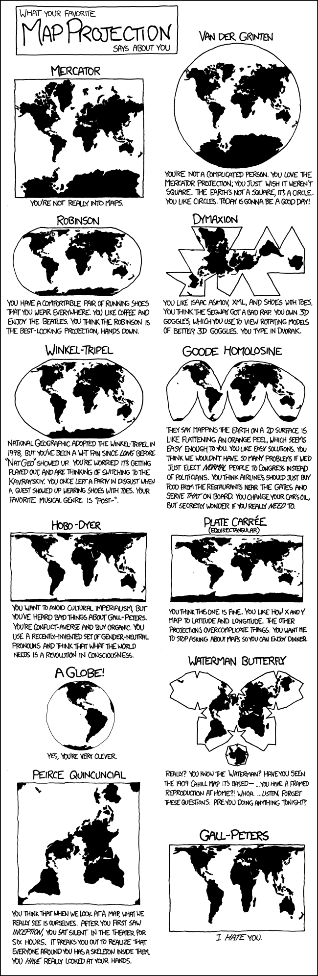
Choosing an appropriate projection for your map is not always straightforward. It depends on what you actually want to represent in your map, and what your data’s spatial scale, resolution and extent are. In fact, there is not a single ‘perfect projection’; each has strengths and weaknesses, and you should choose a projection that fits best for each map. In fact, the projection you choose might even tell something about you:

The XKCD web comic had it figured out long ago: ‘What your favourite map projection tells about you’. Source: xkcd.com

Note

For those of you who prefer a more analytical approach to choosing map projections: you can get a good overview from georeference.org, and this blog post discussing the strengths and weaknesses of a few commonly used projections. The web page Radical Cartography has an excellent overview of which projections fit which extent of the world for which topic.

---

Handling coordinate reference systems in Geopandas

Once you have figured out which map projection to use, handling coordinate reference systems, fortunately, is fairly easy in Geopandas. The library pyproj provides additional information about a CRS, and can assist with more tricky tasks, such as guessing the unknown CRS of a data set.

In this section we will learn how to retrieve the coordinate reference system information of a data set, and how to re-project the data into another CRS.

Careful with Shapefiles

You might have noticed that geospatial data sets in ESRI Shapefile format are consisting of multiple files with different file extensions. The .prj file contains information about the coordinate reference system. Be careful not to lose it!

Displaying the CRS of a data set

We will start by loading a data set of EU countries that has been downloaded from the Geographic Information System of the Commission (GISCO), a unit within Eurostat that manages geospatial data for the European Commission.

import pathlib 
NOTEBOOK_PATH = pathlib.Path().resolve()
DATA_DIRECTORY = NOTEBOOK_PATH / "data"

import geopandas

eu_countries = geopandas.read_file(
    DATA_DIRECTORY / "eu_countries" / "eu_countries_2022.gpkg"
)

Let’s check the data set’s CRS:

eu_countries.crs

<Geographic 2D CRS: EPSG:4326>
Name: WGS 84
Axis Info [ellipsoidal]:
- Lat[north]: Geodetic latitude (degree)
- Lon[east]: Geodetic longitude (degree)
Area of Use:
- name: World.
- bounds: (-180.0, -90.0, 180.0, 90.0)
Datum: World Geodetic System 1984 ensemble
- Ellipsoid: WGS 84
- Prime Meridian: Greenwich

What we see here is, in fact, a pyproj.CRS object.

The EPSG code (European Petroleum Survey Group) is global standard for identifying coordinate reference systems. The number refers to an entry in the EPSG Geodetic Parameter Dataset, a collection of coordinate reference systems coordinate transformations ranging from global to national, regional, and local scope.

Our GeoDataFrame’s EPSG code is 4326. This is number to remember, as you will come across it a lot in the geospatial world: It refers to a geographic coordinate system using the WGS-84 reference ellipsoid. This is the most commonly used coordinate reference system in the world. It’s what we refer to when we speak of longitude and latitude.

You can find information about reference systems and lists of commonly known CRS from many online resources, for example:

• spatialreference.org

• proj4.org

• mapref.org

Tip

If you know what range the coordinate values should be in, it doesn’t hurt to take a quick look at the data itself. In the case of EPSG:4326, coordinates should be between -180 and 180° longitude and -90 and 90° latitude.

eu_countries.geometry.head()

0    MULTIPOLYGON (((13.68400 46.43750, 13.51100 46...
1    MULTIPOLYGON (((6.31560 50.49700, 6.40500 50.3...
2    MULTIPOLYGON (((28.49800 43.43410, 28.06020 43...
3    MULTIPOLYGON (((16.94980 48.53580, 16.85110 48...
4    MULTIPOLYGON (((32.94170 34.64180, 32.55900 34...
Name: geometry, dtype: geometry

Indeed, the coordinate values of our data set seem to be in an appropriate value range.

---

Reprojecting a GeoDataFrame

A geographic coordinate system, EPSG:4326, is not particularly well-suited for showing the countries of the European Union. Distortion is high. Rather, we could use a Lambert Azimuthal Equal-Area projection, such as EPSG:3035, the map projection officially recommended by the European Commission.

Transforming data from one reference system to another is a very simple task in geopandas. In fact, all you have to to is use the to_crs() method of a GeoDataFrame, supplying a new CRS in a wide range of possible formats. The easiest is to use an EPSG code:

eu_countries_EPSG3035 = eu_countries.to_crs("EPSG:3035")

Let’s check how the coordinate values have changed:

eu_countries_EPSG3035.geometry.head()

0    MULTIPOLYGON (((4604288.477 2598607.470, 45914...
1    MULTIPOLYGON (((4059689.242 3049361.180, 40650...
2    MULTIPOLYGON (((5805367.757 2442801.252, 57739...
3    MULTIPOLYGON (((4833567.363 2848881.974, 48272...
4    MULTIPOLYGON (((6413299.362 1602181.345, 63782...
Name: geometry, dtype: geometry

And here we go, the coordinate values in the geometries have changed! Congratulations on carrying out your very first geopandas coordinate transformation!

To better grasp what exactly we have just done, it is a good idea to explore our data visually. Let’s plot our data set both before and after the coordinate transformation. We will use matplotlib’s subplots feature that we got to know in Geo-Python lesson 7.

import matplotlib.pyplot

# Prepare sub plots that are next to each other
figure, (axis1, axis2) = matplotlib.pyplot.subplots(nrows=1, ncols=2)

# Plot the original (WGS84, EPSG:4326) data set
eu_countries.plot(ax=axis1)
axis1.set_title("WGS84")
axis1.set_aspect(1)

# Plot the reprojected (EPSG:3035) data set
eu_countries_EPSG3035.plot(ax=axis2)
axis2.set_title("ETRS-LAEA")
axis2.set_aspect(1)

matplotlib.pyplot.tight_layout()

Indeed, the maps look quite different, and the re-projected data set distorts the European countries less, especially in the Northern part of the continent.

Let’s still save the reprojected data set in a file so we can use it later. Note that, even though modern file formats save the CRS reliably, it is a good idea to use a descriptive file name that includes the reference system information.

eu_countries_EPSG3035.to_file(
    DATA_DIRECTORY / "eu_countries" / "eu_countries_EPSG3035.gpkg"
)

---

Handling different CRS formats

There are different ways to store and represent CRS information. The more commonly used formats include PROJ strings, EPSG codes, Well-Known-Text (WKT) and JSON. You will likely encounter some or all of these when working with spatial data obtained from different sources. Being able to convert CRS information from one format to another is needed every now and then, hence, it is useful to know a few tricks how to do this.

We’ve already briefly mentioned that geopandas uses the pyproj library to handle reference systems. We can use the same module to parse and convert CRS information in different formats.

Overview

Below we print different representations of the CRS of the data set of EU countries we used before:

import pyproj

crs = pyproj.CRS(eu_countries.crs)

print(f"CRS as a proj4 string: {crs.to_proj4()}\n")

print(f"CRS in WKT format: {crs.to_wkt()}\n")

print(f"EPSG code of the CRS: {crs.to_epsg()}\n")

CRS as a proj4 string: +proj=longlat +datum=WGS84 +no_defs +type=crs

CRS in WKT format: GEOGCRS["WGS 84",ENSEMBLE["World Geodetic System 1984 ensemble",MEMBER["World Geodetic System 1984 (Transit)"],MEMBER["World Geodetic System 1984 (G730)"],MEMBER["World Geodetic System 1984 (G873)"],MEMBER["World Geodetic System 1984 (G1150)"],MEMBER["World Geodetic System 1984 (G1674)"],MEMBER["World Geodetic System 1984 (G1762)"],MEMBER["World Geodetic System 1984 (G2139)"],ELLIPSOID["WGS 84",6378137,298.257223563,LENGTHUNIT["metre",1]],ENSEMBLEACCURACY[2.0]],PRIMEM["Greenwich",0,ANGLEUNIT["degree",0.0174532925199433]],CS[ellipsoidal,2],AXIS["geodetic latitude (Lat)",north,ORDER[1],ANGLEUNIT["degree",0.0174532925199433]],AXIS["geodetic longitude (Lon)",east,ORDER[2],ANGLEUNIT["degree",0.0174532925199433]],USAGE[SCOPE["Horizontal component of 3D system."],AREA["World."],BBOX[-90,-180,90,180]],ID["EPSG",4326]]

EPSG code of the CRS: 4326

/home/docs/checkouts/readthedocs.org/user_builds/autogis-site/envs/latest/lib/python3.10/site-packages/pyproj/crs/crs.py:1286: UserWarning: You will likely lose important projection information when converting to a PROJ string from another format. See: https://proj.org/faq.html#what-is-the-best-format-for-describing-coordinate-reference-systems
  proj = self._crs.to_proj4(version=version)

Note

Not every possible coordinate reference system has an EPSG code assigned. That’s why pyproj, by default, tries to find the best-matching EPSG definition. If it does not find any, to_epsg() returns None.

Use pyproj to find detailed information about a CRS

A pyproj.CRS object can also be initialised manually, for instance, using an EPSG code or a Proj4-string. It can then provide detailed information on the parameters of the reference system, as well as suggested areas of use. We can, for example, create a CRS object for the EPSG:3035 map projection we used above:

crs = pyproj.CRS("EPSG:4326")
crs

<Geographic 2D CRS: EPSG:4326>
Name: WGS 84
Axis Info [ellipsoidal]:
- Lat[north]: Geodetic latitude (degree)
- Lon[east]: Geodetic longitude (degree)
Area of Use:
- name: World.
- bounds: (-180.0, -90.0, 180.0, 90.0)
Datum: World Geodetic System 1984 ensemble
- Ellipsoid: WGS 84
- Prime Meridian: Greenwich

Immediately, we see that a pyproj.CRS object contains rich information about the reference system: a name, an area of use (including bounds), a datum and an ellipsoid.

This information can also be extraced individually:

crs.name

'WGS 84'

crs.area_of_use.bounds

(-180.0, -90.0, 180.0, 90.0)

---

Global map projections

Finally, it’s time to play around with some map projections. For this, you will find a global data set of country polygons in the data directory. It was downloaded from naturalearthdata.com, a fantastic resource for cartographer-grade geodata.

Check your understanding

Read in the data set from DATA_DIRECTORY / "world_countries" / "ne_110m_admin_0_countries.zip" and plot three maps with different map projections. You can use the hints and definitions from the following resources (and anywhere else):

• geopandas.org/projections.html

• pyproj4.github.io

• spatialreference.org

While plotting the maps and choosing map projections, think about the advantages and disavantages of different map projections.

world_countries = geopandas.read_file(
    DATA_DIRECTORY / "world_countries" / "ne_110m_admin_0_countries.zip"
)

world_countries.plot()
matplotlib.pyplot.title(world_countries.crs.name)

Text(0.5, 1.0, 'WGS 84')

# web mercator
world_countries_EPSG3857 = world_countries.to_crs("EPSG:3857")

world_countries_EPSG3857.plot()
matplotlib.pyplot.title(world_countries_EPSG3857.crs.name)

# remove axis decorations
matplotlib.pyplot.axis("off")

(-22041259.17706817,
 22041259.177068174,
 -255577115.13568556,
 31488437.087057084)

# Eckert-IV (https://spatialreference.org/ref/esri/54012/)
ECKERT_IV = "+proj=eck4 +lon_0=0 +x_0=0 +y_0=0 +ellps=WGS84 +datum=WGS84 +units=m +no_defs"

world_countries_eckert_iv = world_countries.to_crs(ECKERT_IV)
world_countries_eckert_iv.plot()
matplotlib.pyplot.title("Eckert Ⅳ")
matplotlib.pyplot.axis("off")

(-18321736.696081996,
 18321736.696081996,
 -9302420.503183275,
 9217598.414473996)

# An orthographic projection, centered in Finland!
# (http://www.statsmapsnpix.com/2019/09/globe-projections-and-insets-in-qgis.html)
world_countries_ortho = world_countries.to_crs(
    "+proj=ortho +lat_0=60.00 +lon_0=23.0000 +x_0=0 +y_0=0 "
    "+a=6370997 +b=6370997 +units=m +no_defs"
)
world_countries_ortho.plot()
matplotlib.pyplot.axis("off")

(-7006995.416935118, 7005877.340582642, -6968264.187936907, 6378854.706416504)