Introduction to Geopandas¶

Geopandas (http://geopandas.org/) makes it possible to work with geospatial data in Python in a relatively easy way. Geopandas combines the capabilities of the data analysis library pandas with other packages like shapely and fiona for managing spatial data.

The main data structures in geopandas; GeoSeries and GeoDataFrame extend the capabilities of Series and DataFrames from pandas. This means that we can apply our pandas skills also with geopandas data structures. If you need to refresh your memory about pandas, check out week 5 and 6 lesson materials from the Geo-Python website.

The main difference between geodataframes and pandas dataframes is that a geodataframe should contain one column for geometries (by default, the name of this column is 'geometry'). The geometry column is a geoseries which contains the geometries (points, lines, polygons, multipolygons etc.) for each row of data.

As we learned in the Geo-Python course, it is conventional to import pandas as pd. Similarly,we will import geopandas as gpd:

import geopandas as gpd

In this lesson, we will cover basics steps needed for interacting with spatial data in Python using geopandas:

Managing filepaths
Reading a shapefile
Geometry calculations
Writing a shapefile
Grouping and splitting spatial data into multiple layers

Before diving deeper into geopandas functionalities, let’s first acquire some input data to work with.

Input data: Finnish topographic database¶

Topographic Database from the National Land Survey of Finland (NLS).
The data set is licensed under the NLS’ open data licence (CC BY 4.0).
Structure of the data is described in a separate Excel file (download link).
Further information about file naming at fairdata.fi.
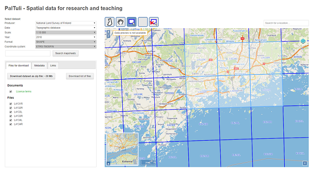
We acquired the data via the CSC open data portal:

Paituli data download

In this lesson, we will focus on terrain objects (Feature group: “Terrain/1”) downloaded as Shapefiles. According to the naming convention of the Topographic Database for Shapefiles, all files that start with a letter m and end with p contain the objects we are interested in (Terrain/1 polygons). Furthermore, the Terrain/1 feature group contains several feature classes. Our final task in this lesson is to save all these feature classes into separate files.

Terrain/1 features in the Topographic Database:

feature class	Name of feature	Feature group
32421	Motor traffic area	Terrain/1
32200	Cemetery	Terrain/1
34300	Sand	Terrain/1
34100	Rock - area	Terrain/1
34700	Rocky area	Terrain/1
32500	Quarry	Terrain/1
32112	Mineral resources extraction area, fine-grained material	Terrain/1
32111	Mineral resources extraction area, coarse-grained material	Terrain/1
32611	Field	Terrain/1
32612	Garden	Terrain/1
32800	Meadow	Terrain/1
32900	Park	Terrain/1
35300	Paludified land	Terrain/1
35412	Bog, easy to traverse forested	Terrain/1
35411	Open bog, easy to traverse treeless	Terrain/1
35421	Open fen, difficult to traverse treeless	Terrain/1
33000	Earth fill	Terrain/1
33100	Sports and recreation area	Terrain/1
36200	Lake water	Terrain/1
36313	Watercourse area	Terrain/1

Downloading data¶

On Binder and CSC Notebook environment, you can use wget program to download the data from the command line. Let’s download the data (download link) into the same folder with the lesson 2 notebooks (.../notebooks/L2):

Open up a new terminal window
Navigate to the correct folder in the terminal:

# Navigate to lesson 2 notebooks directory:
$ cd /home/jovyan/work/autogis/notebooks/notebooks/L2
    

use wget utility to dowload the data from the dowload link:

$ wget https://github.com/AutoGIS/data/raw/master/L2_data.zip

Copy-paste

You can copy/paste things to JupyterLab Terminal by pressing SHIFT + RIGHT-CLICK on your mouse and choosing Paste.

Once you have downloaded the L2_data.zip file into your home directory, you can unzip the file using unzip command in the Terminal (or e.g. 7zip on Windows if working with own computer). Run the following commands in the .../notebooks/L2 -directory:

$ unzip L2_data.zip
$ ls L2_data

You can also check the contents of the downloaded and unzipped file in the file browser window.

The L2_data folder contains several subfolders. After unzipping the downloaded file, you can find the data for this tutorial under: L2_data/NLS/2018/L4/L41/L4132R.shp. Notice that Shapefile -fileformat contains many separate files such as .dbf that contains the attribute information, and .prj -file that contains information about coordinate reference system.

Managing filepaths¶

Built-in module os provides many useful functions for interacting with the operating system. One of the most useful submodules in the os package is the os.path-module for manipulating file paths. This week, we have data in different sub-folders and we can practice how to use os path tools when defining filepaths.

Let’s import os and see how we can construct a filepath by joining a folder path and file name:

import os

# Define path to folder
input_folder = r"L2_data/NLS/2018/L4/L41/L4132R.shp"

# Join folder path and filename 
fp = os.path.join(input_folder, "m_L4132R_p.shp")

# Print out the full file path
print(fp)

L2_data/NLS/2018/L4/L41/L4132R.shp/m_L4132R_p.shp

Reading a Shapefile¶

Typically reading the data into Python is the first step of the analysis pipeline. There are various different GIS data formats available. Shapefile, GeoJSON, KML, and GPKG are one of the most common vector data formats currently in use. Geopandas is capable of reading data from all of these formats (plus many more).

In geopandas, we use a generic function .from_file() for reading in different data formats. In the bacground, Geopandas uses fiona.open() when reading in data.

When reading in a Shapefile, we only need to pass the filepath when reading data:

import geopandas as gpd

# Read file using gpd.read_file()
data = gpd.read_file(fp)

Let’s see check the data type:

type(data)

geopandas.geodataframe.GeoDataFrame

Here we see that our data -variable is a GeoDataFrame. GeoDataFrame extends the functionalities of pandas.DataFrame in a way that it is possible to handle spatial data using similar approaches and datastructures as in pandas (hence the name geopandas).

Let’s take a look at our data and print the first rows using the head() -function:

print(data.head())

  TEKSTI  RYHMA  LUOKKA  TASTAR  KORTAR  KORARV  KULKUTAPA    KOHDEOSO  \
 None     64   32421    5000       0     0.0          0  1812247077   
 None     64   32421    5000       0     0.0          0  1718796908   
 None     64   32421   20000       0     0.0          0   411167695   
 None     64   32421   20000       0     0.0          0   411173768   
 None     64   32421   20000       0     0.0          0   411173698   

   AINLAHDE SYNTYHETKI  ... KARTOGLK  ALUEJAKOON  VERSUH  SUUNTA  SIIRT_DX  \
       1   20180125  ...        0           0       0       0         0   
       1   20180120  ...        0           0       0       0         0   
       1   20180120  ...        0           0       0       0         0   
       1   20180120  ...        0           0       0       0         0   
       1   20180120  ...        0           0       0       0         0   

   SIIRT_DY  KORKEUS  ATTR2  ATTR3  \
       0      0.0      0      0   
       0      0.0      0      0   
       0      0.0      0      0   
       0      0.0      0      0   
       0      0.0      0      0   

                                            geometry  
POLYGON ((379394.248 6689991.936, 379389.790 6...  
POLYGON ((378980.811 6689359.377, 378983.401 6...  
POLYGON ((378804.766 6689256.471, 378817.107 6...  
POLYGON ((379229.695 6685025.111, 379233.366 6...  
POLYGON ((379825.199 6685096.247, 379829.651 6...  

[5 rows x 21 columns]

Check all column names:

data.columns

Index(['TEKSTI', 'RYHMA', 'LUOKKA', 'TASTAR', 'KORTAR', 'KORARV', 'KULKUTAPA',
       'KOHDEOSO', 'AINLAHDE', 'SYNTYHETKI', 'KUOLHETKI', 'KARTOGLK',
       'ALUEJAKOON', 'VERSUH', 'SUUNTA', 'SIIRT_DX', 'SIIRT_DY', 'KORKEUS',
       'ATTR2', 'ATTR3', 'geometry'],
      dtype='object')

As most of you probably notice, all the column names are in Finnish…

Let’s select only the useful columns and rename them into English:

data = data[['RYHMA', 'LUOKKA',  'geometry']]

Define new column names in a dictionary:

colnames = {'RYHMA':'GROUP', 'LUOKKA':'CLASS'}

rename the columns:

data.rename(columns=colnames, inplace=True)

data.columns

Index(['GROUP', 'CLASS', 'geometry'], dtype='object')

Task

Figure out the following information from our input data based on your pandas-skills from the Geo-Python course:

Number of rows?
Number of classes?
Number of groups?

Solutions:

print("Number of rows", len(data['CLASS']))
print("Number of classes", data['CLASS'].nunique())
print("Number of groups", data['GROUP'].nunique())

Number of rows 4311
Number of classes 20
Number of groups 1

It is always a good idea to explore your data also on a map. Creating a simple map from a GeoDataFrame is really easy: you can use .plot() -function from geopandas that creates a map based on the geometries of the data. Geopandas actually uses matplotlib for plotting which we introduced in Lesson 7 of the Geo-Python course.

Let’s try it out, and plot our GeoDataFrame:

%matplotlib inline
data.plot()

<matplotlib.axes._subplots.AxesSubplot at 0x7f8cc41d46a0>

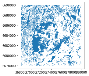
Voilá! As we can see, it is really easy to produce a map out of your Shapefile with geopandas. Geopandas automatically positions your map in a way that it covers the whole extent of your data.

If you are living in the Helsinki region, you might recognize the shapes plotted on the map!

Geometries in Geopandas¶

Geopandas takes advantage of Shapely’s geometric objects. Geometries are stored in a column called geometry that is a default column name for storing geometric information in geopandas.

Let’s print the first 5 rows of the column ‘geometry’:

# It is possible to get a specific column by specifying the column name within square brackets []
print(data['geometry'].head())

  POLYGON ((379394.248 6689991.936, 379389.790 6...
  POLYGON ((378980.811 6689359.377, 378983.401 6...
  POLYGON ((378804.766 6689256.471, 378817.107 6...
  POLYGON ((379229.695 6685025.111, 379233.366 6...
  POLYGON ((379825.199 6685096.247, 379829.651 6...
Name: geometry, dtype: geometry

As we can see the geometry column contains familiar looking values, namely Shapely Polygon -objects. Since the spatial data is stored as Shapely objects, it is possible to use all of the functionalities of the Shapely module when dealing with geometries in geopandas.

Let’s have a closer look at the polygons and try to apply some of the Shapely methods we learned last week.

Let’s start by checking the area of the first polygon in the data:

print("Polygon:", data.at[0, "geometry"])
print("Area:", round(data.at[0, "geometry"].area,0), "square meters")

Polygon: POLYGON ((379394.248 6689991.936, 379389.79 6690000, 379408.646 6690000, 379394.248 6689991.936))
Area: 76.0 square meters

Let’s do the same for the first five rows in the data;

Iterate over the GeoDataFrame rows using the iterrows() -function that we learned during the Lesson 6 of the Geo-Python course.
For each row, print the area of the polygon (here, we’ll limit the for-loop to a selection of the first five rows):

# Iterate over rows and print the area of a Polygon
for index, row in data[0:5].iterrows():
    
    # Get the area from the shapely-object stored in the geometry-column
    poly_area = row['geometry'].area
    
    # Print info
    print("Polygon area at index {index} is: {area:.2f} m^2".format(index=index, area=poly_area))

Polygon area at index 0 is: 76.03 m^2
Polygon area at index 1 is: 2652.05 m^2
Polygon area at index 2 is: 3185.65 m^2
Polygon area at index 3 is: 13075.17 m^2
Polygon area at index 4 is: 3980.68 m^2

As you see from here, all the functionalities of pandas, such as the iterrows() function, are directly available in Geopandas without the need to call pandas separately because Geopandas is an extension for pandas.

In practice, it is not necessary to use the iterrows()-approach to calculate the area for all features. Geodataframes and geoseries have an attribute area which we can use for accessing the area for each feature at once:

data.area.head()

     76.027392
   2652.054186
   3185.649995
  13075.165279
   3980.682621
dtype: float64

Let’s next create a new column into our GeoDataFrame where we calculate and store the areas of individual polygons:

# Create a new column called 'area' and assign the area of the Polygons into it
data['area'] = data.area

Check the output:

data['area'].head()

     76.027392
   2652.054186
   3185.649995
  13075.165279
   3980.682621
Name: area, dtype: float64

These values correspond to the ones we saw in previous step when iterating rows.

Let’s check what is the min, max and mean of those areas using familiar functions from our previous Pandas lessions.

# Maximum area
max_area = data['area'].max()

# Minimum area
min_area = data['area'].min()

# Mean area
mean_area = data['area'].mean()

print("Max area: {maximum} square meters".format(maximum=round(max_area, 0)))
print("Min area: {minimum} square meters".format(minimum=round(min_area, 0)))
print("Mean area: {mean} square meters".format(mean=round(mean_area, 0)))

Max area: 4084558.0 square meters
Min area: 1.0 square meters
Mean area: 11522.0 square meters

Writing a shapefile¶

It is possible to export GeoDataFrames into various data formats using gpd.to_file(). Here, we will first learn how to export a subset of the data into a Shapefile.

Let’s first select one class (class number 36200, “Lake water”) from the data as a new GeoDataFrame:

# Select a class
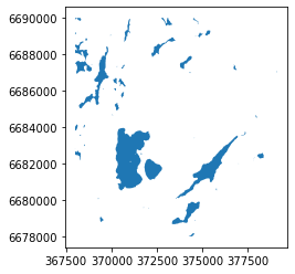
selection = data.loc[data["CLASS"]==36200]

Check the selection:

selection.plot()

<matplotlib.axes._subplots.AxesSubplot at 0x7f8cc4199710>

write this layer into a new Shapefile using the gpd.to_file() -function:

# Create a output path for the data
output_folder = r"L2_data/"
output_fp = os.path.join(output_folder, "Class_36200.shp")

# Write those rows into a new file (the default output file format is Shapefile)
selection.to_file(output_fp)

Task

Read the output Shapefile in a new geodataframe, and check that the data looks ok.

Grouping the Geodataframe¶

One really useful function that can be used in Pandas/Geopandas is .groupby() which groups data based on values on selected column(s). We saw and used this function already in Lesson 6 of the Geo-Python course.

Next we will automate the file export task; we will group the data based on column CLASS and export a shapefile for each class.

Let’s continue with the same input file we already read previously into the variable data. We also selected and renamed a subset of the columns.

Check the first rows of the data:

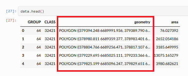
data.head()

	GROUP	CLASS	geometry	area
0	64	32421	POLYGON ((379394.248 6689991.936, 379389.790 6...	76.027392
1	64	32421	POLYGON ((378980.811 6689359.377, 378983.401 6...	2652.054186
2	64	32421	POLYGON ((378804.766 6689256.471, 378817.107 6...	3185.649995
3	64	32421	POLYGON ((379229.695 6685025.111, 379233.366 6...	13075.165279
4	64	32421	POLYGON ((379825.199 6685096.247, 379829.651 6...	3980.682621

The CLASS column in the data contains information about different land use types. With .unique() -function we can quickly see all different values in that column:

# Print all unique values in the column
print(data['CLASS'].unique())

[32421 32200 34300 34100 34700 32500 32112 32111 32611 32612 32800 32900
 35300 35412 35411 35421 33000 33100 36200 36313]

Now we can use that information to group our data and save all land use types into different layers:

# Group the data by class
grouped = data.groupby('CLASS')

# Let's see what we have
grouped

<pandas.core.groupby.generic.DataFrameGroupBy object at 0x7f8cc4175048>

As we can see, groupby -function gives us an object called DataFrameGroupBy which is similar to list of keys and values (in a dictionary) that we can iterate over. For more information about grouped objects, see Lesson 6 of the Geo-Python course.

Check out all group keys:

grouped.groups.keys()

dict_keys([32111, 32112, 32200, 32421, 32500, 32611, 32612, 32800, 32900, 33000, 33100, 34100, 34300, 34700, 35300, 35411, 35412, 35421, 36200, 36313])

The group keys are unique values from the column by which we grouped the dataframe.

Check how many rows of data each group has:

# Iterate over the group object
for key, group in grouped:

    # Let's check how many rows each group has:
    print('Terrain class:', key)
    print('Number of rows:', len(group), "\n")

Terrain class: 32111
Number of rows: 1 

Terrain class: 32112
Number of rows: 1 

Terrain class: 32200
Number of rows: 2 

Terrain class: 32421
Number of rows: 110 

Terrain class: 32500
Number of rows: 2 

Terrain class: 32611
Number of rows: 257 

Terrain class: 32612
Number of rows: 11 

Terrain class: 32800
Number of rows: 80 

Terrain class: 32900
Number of rows: 28 

Terrain class: 33000
Number of rows: 5 

Terrain class: 33100
Number of rows: 118 

Terrain class: 34100
Number of rows: 3005 

Terrain class: 34300
Number of rows: 1 

Terrain class: 34700
Number of rows: 3 

Terrain class: 35300
Number of rows: 134 

Terrain class: 35411
Number of rows: 35 

Terrain class: 35412
Number of rows: 449 

Terrain class: 35421
Number of rows: 5 

Terrain class: 36200
Number of rows: 56 

Terrain class: 36313
Number of rows: 8 

There are, for example, 56 lake polygons in the input data.

We can also check how the last group looks like (we have the variables in memory from the last iteration of the for-loop):

group.head()

	GROUP	CLASS	geometry	area
4303	64	36313	POLYGON ((377127.305 6688073.257, 377116.045 6...	9619.307973
4304	64	36313	POLYGON ((371141.897 6677999.999, 371139.757 6...	25266.167705
4305	64	36313	POLYGON ((371498.720 6680399.799, 371497.585 6...	364.087680
4306	64	36313	POLYGON ((375668.607 6682942.062, 375671.489 6...	2651.800270
4307	64	36313	POLYGON ((368411.063 6679328.990, 368411.424 6...	376.503380

Notice that the index numbers refer to the row numbers in the original data -GeoDataFrame.

Check also the data type of the group:

type(group)

geopandas.geodataframe.GeoDataFrame

As we can see, each set of data are now grouped into separate GeoDataFrames, and we can save them into separate files.

Saving multiple output files¶

Let’s export each class into a separate Shapefile. While doing this, we also want to create unique filenames for each class.

When looping over the grouped object, information about the class is stored in the variable key, and we can use this information for creating new variable names inside the for-loop. For example, we want to name the shapefile containing lake polygons as “terrain_36200.shp”.

String formatting

There are different approaches for formatting strings in Python. Here are a couple of different ways for putting together file-path names using two variables:

basename = "terrain"
key = 36200

# OPTION 1. Concatenating using the `+` operator:
out_fp = basename + "_" + str(key) + ".shp"

# OPTION 2. Positional formatting using `%` operator
out_fp = "%s_%s.shp" %(basename, key)
    
# OPTION 3. Positional formatting using `.format()`
out_fp = "{}_{}.shp".format(basename, key)

Read more from here: https://pyformat.info/

Let’s now export terrain classes into separate Shapefiles.

First, create a new folder for the outputs:

# Determine output directory
output_folder = r"L2_data/"

# Create a new folder called 'Results' 
result_folder = os.path.join(output_folder, 'Results')

# Check if the folder exists already
if not os.path.exists(result_folder):
    # If it does not exist, create one
    os.makedirs(result_folder)

At this point, you can go to the file browser and check that the new folder was created successfully.

Iterate over groups, create a file name, and save group to file:

# Iterate over the groups
for key, group in grouped:
    # Format the filename 
    output_name = "terrain_%s.shp" % str(key)

    # Print information about the process
    print("Saving file", os.path.basename(output_name))

    # Create an output path
    outpath = os.path.join(result_folder, output_name)

    # Export the data
    group.to_file(outpath)

Saving file terrain_32111.shp
Saving file terrain_32112.shp
Saving file terrain_32200.shp
Saving file terrain_32421.shp
Saving file terrain_32500.shp
Saving file terrain_32611.shp
Saving file terrain_32612.shp
Saving file terrain_32800.shp
Saving file terrain_32900.shp
Saving file terrain_33000.shp
Saving file terrain_33100.shp
Saving file terrain_34100.shp
Saving file terrain_34300.shp
Saving file terrain_34700.shp
Saving file terrain_35300.shp
Saving file terrain_35411.shp
Saving file terrain_35412.shp
Saving file terrain_35421.shp
Saving file terrain_36200.shp
Saving file terrain_36313.shp

Excellent! Now we have saved those individual classes into separate Shapefiles and named the file according to the class name. These kind of grouping operations can be really handy when dealing with layers of spatial data. Doing similar process manually would be really laborious and error-prone.

Extra: save data to csv¶

We can also extract basic statistics from our geodataframe, and save this information as a text file.

Let’s summarize the total area of each group:

area_info = grouped.area.sum().round()

area_info

CLASS
      1834.0
      2148.0
    105737.0
    702073.0
    109747.0
  13135597.0
    107343.0
   1465278.0
    617209.0
    659465.0
   3777595.0
  12381611.0
      1627.0
      2786.0
   1382940.0
    411198.0
   4710133.0
     67864.0
   9986966.0
     43459.0
Name: area, dtype: float64

save area info to csv using pandas:

# Create an output path
area_info.to_csv("terrain_class_areas.csv", header=True)

Summary¶

In this tutorial we introduced the first steps of using geopandas. More specifically you should know how to:

Read data from Shapefile using geopandas
Access geometry information in a geodataframe
Write GeoDataFrame data from Shapefile using geopandas
Automate a task to save specific rows from data into Shapefile based on specific key using groupby() -function
Extra: saving attribute information to a csv file.