Raster map algebra
Conducting calculations between bands or raster is another common GIS task. Here, we will be calculating NDVI (Normalized difference vegetation index) based on the Landsat dataset that we have downloaded from Helsinki region. Conducting calculations with rasterio is fairly straightforward if the extent etc. matches because the values of the rasters are stored as numpy arrays (similar to the columns stored in Geo/Pandas, i.e. Series).
Calculating NDVI
In this tutorial, we will see how to calculate the NDVI (Normalized difference vegetation index) based on two bands: band-4 which is the Red channel and band-5 which is the Near Infrared (NIR).
Let’s start by importing the necessary modules
rasterioandnumpyand reading the raster file that we masked for Helsinki Region:
import rasterio
import numpy as np
from rasterio.plot import show
import os
import matplotlib.pyplot as plt
%matplotlib inline

# Data dir
data_dir = "data"

# Filepath
fp = os.path.join(data_dir, "Helsinki_masked_p188r018_7t20020529_z34__LV-FIN.tif")

# Open the raster file in read mode
raster = rasterio.open(fp)
Let’s read the red and NIR bands from our raster source (ref):
# Read red channel (channel number 3)
red = raster.read(3)
# Read NIR channel (channel number 4)
nir = raster.read(4)
# Calculate some stats to check the data
print(red.mean())
print(nir.mean())
print(type(nir))
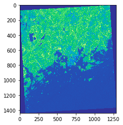
# Visualize
show(nir, cmap='terrain')
36.29418775547201
35.0946303937776
<class 'numpy.ndarray'>
<matplotlib.axes._subplots.AxesSubplot at 0x251e87acc88>
As we can see the values are stored as numpy.ndarray. From the map we can see that NIR channel reflects stronly (light green) in areas outside the Helsinki urban areas.
Let’s change the data type from uint8 to float so that we can have floating point numbers stored in our arrays:
# Convert to floats
red = red.astype('f4')
nir = nir.astype('f4')
nir
array([[0., 0., 0., ..., 0., 0., 0.],
       [0., 0., 0., ..., 0., 0., 0.],
       [0., 0., 0., ..., 0., 0., 0.],
       ...,
       [0., 0., 0., ..., 0., 0., 0.],
       [0., 0., 0., ..., 0., 0., 0.],
       [0., 0., 0., ..., 0., 0., 0.]], dtype=float32)
Now we can see that the numbers changed to decimal numbers (there is a dot after the zero).
Next we need to tweak the behaviour of numpy a little bit. By default numpy will complain about dividing with zero values. We need to change that behaviour because we have a lot of 0 values in our data.
np.seterr(divide='ignore', invalid='ignore')
{'divide': 'warn', 'over': 'warn', 'under': 'ignore', 'invalid': 'warn'}
Now we are ready to calculate the NDVI. This can be done easily with simple map algebra and using the NDVI formula and passing our numpy arrays into it:
# Calculate NDVI using numpy arrays
ndvi = (nir - red) / (nir + red)
Let’s plot the results so we can see how the index worked out:
%matplotlib inline
# Plot the NDVI
plt.imshow(ndvi, cmap='terrain_r')
# Add colorbar to show the index
plt.colorbar()
<matplotlib.colorbar.Colorbar at 0x251e889f9e8>
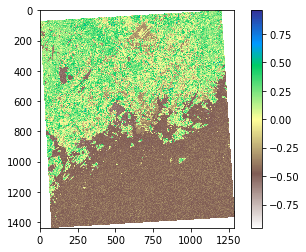
As we can see from the map, now the really low NDVI indices are located in water and urban areas (middle of the map) whereas the areas colored with green have a lot of vegetation according our NDVI index.