Zonal statistics¶

Quite often you have a situtation when you want to summarize raster datasets based on vector geometries, such as calculating the average elevation of specific area.

Rasterstats is a Python module that does exactly that, easily.

Let’s start by reading the data:

import rasterio
from rasterio.plot import show
from rasterstats import zonal_stats
import osmnx as ox
import geopandas as gpd
import os
import matplotlib.pyplot as plt
%matplotlib inline

# File path
data_dir = "L5_data"
dem_fp = os.path.join(data_dir, "Helsinki_DEM2x2m_Mosaic.tif")

# Read the Digital Elevation Model for Helsinki
dem = rasterio.open(dem_fp)
dem

<open DatasetReader name='L5_data\Helsinki_DEM2x2m_Mosaic.tif' mode='r'>

Good, now our elevation data is in read mode.

Next, we want to calculate the elevation of two neighborhoods located in Helsinki, called Kallio and Pihlajamäki, and find out which one of them is higher based on the elevation data. We will use a package called OSMnx to fetch the data from OpenStreetMap for those areas.

Specify place names for Kallio and Pihlajamäki that Nominatim can identify https://nominatim.openstreetmap.org/, and retrieve the

# Keywords for Kallio and Helsinki in such format that they can be found from OSM
kallio_q = "Kallio, Helsinki, Finland"
pihlajamaki_q = "Pihlajamäki, Malmi, Helsinki, Finland"

# Retrieve the geometries of those areas using osmnx
kallio = ox.gdf_from_place(kallio_q)
pihlajamaki = ox.gdf_from_place(pihlajamaki_q)

# Reproject to same coordinate system as the 
kallio = kallio.to_crs(crs=dem.crs)
pihlajamaki = pihlajamaki.to_crs(crs=dem.crs)

type(kallio)

geopandas.geodataframe.GeoDataFrame

As we can see, now we have retrieved data from OSMnx and they are stored as GeoDataFrames.

Let’s see how our datasets look by plotting the DEM and the regions on top of it

# Plot the Polygons on top of the DEM
ax = kallio.plot(facecolor='None', edgecolor='red', linewidth=2)
ax = pihlajamaki.plot(ax=ax, facecolor='None', edgecolor='blue', linewidth=2)

# Plot DEM
show((dem, 1), ax=ax)

<matplotlib.axes._subplots.AxesSubplot at 0x17a78864c18>

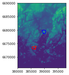
Which one is higher? Kallio or Pihlajamäki? We can use zonal statistics to find out!

First we need to get the values of the dem as numpy array and the affine of the raster

# Read the raster values
array = dem.read(1)

# Get the affine
affine = dem.transform

Now we can calculate the zonal statistics by using the function zonal_stats.

# Calculate zonal statistics for Kallio
zs_kallio = zonal_stats(kallio, array, affine=affine, stats=['min', 'max', 'mean', 'median', 'majority'])

# Calculate zonal statistics for Pihlajamäki
zs_pihla = zonal_stats(pihlajamaki, array, affine=affine, stats=['min', 'max', 'mean', 'median', 'majority'])

C:\ProgramData\Anaconda3\lib\site-packages\rasterstats\io.py:294: UserWarning: Setting nodata to -999; specify nodata explicitly
  warnings.warn("Setting nodata to -999; specify nodata explicitly")

Okey. So what do we have now?

print(zs_kallio)
print(zs_pihla)

[{'min': -2.1760001182556152, 'max': 37.388999938964844, 'mean': 12.759059456081534, 'median': 11.267999649047852, 'majority': 0.3490000069141388}]
[{'min': 8.73799991607666, 'max': 46.30400085449219, 'mean': 24.560033970865877, 'median': 24.17300033569336, 'majority': 10.41100025177002}]

Super! Now we can see that Pihlajamäki seems to be slightly higher compared to Kallio.