Read Cloud Optimized Geotiffs
The following materials are based on this tutorial. Read more from that tutorial until this one get’s better updated.
Let’s read a Landsat TIF profile from AWS cloud storage:
import rasterio
import matplotlib.pyplot as plt
import numpy as np

# Specify the path for Landsat TIF on AWS
fp = 'http://landsat-pds.s3.amazonaws.com/c1/L8/042/034/LC08_L1TP_042034_20170616_20170629_01_T1/LC08_L1TP_042034_20170616_20170629_01_T1_B4.TIF'

# See the profile
with rasterio.open(fp) as src:
    print(src.profile)
{'driver': 'GTiff', 'dtype': 'uint16', 'nodata': None, 'width': 7821, 'height': 7951, 'count': 1, 'crs': CRS({'init': 'epsg:32611'}), 'transform': Affine(30.0, 0.0, 204285.0,
       0.0, -30.0, 4268115.0), 'blockxsize': 512, 'blockysize': 512, 'tiled': True, 'compress': 'deflate', 'interleave': 'band'}
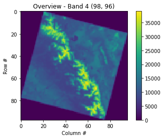
Let’s plot a low resolution overview:
%matplotlib inline
# Open the COG
with rasterio.open(fp) as src:
    # List of overviews from biggest to smallest
    oviews = src.overviews(1)

    # Retrieve the smallest thumbnail
    oview = oviews[-1]
    print('Decimation factor= {}'.format(oview))
    # NOTE this is using a 'decimated read' (http://rasterio.readthedocs.io/en/latest/topics/resampling.html)
    thumbnail = src.read(1, out_shape=(1, int(src.height // oview), int(src.width // oview)))

print('array type: ',type(thumbnail))
print(thumbnail)

plt.imshow(thumbnail)
plt.colorbar()
plt.title('Overview - Band 4 {}'.format(thumbnail.shape))
plt.xlabel('Column #')
plt.ylabel('Row #')
Decimation factor= 81
array type:  <class 'numpy.ndarray'>
[[0 0 0 ..., 0 0 0]
 [0 0 0 ..., 0 0 0]
 [0 0 0 ..., 0 0 0]
 ...,
 [0 0 0 ..., 0 0 0]
 [0 0 0 ..., 0 0 0]
 [0 0 0 ..., 0 0 0]]
<matplotlib.text.Text at 0x1b6fdc750f0>
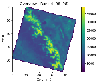
Let’s fix the NoData values to be
NaNinstead of 0:
# Open the file
with rasterio.open(fp) as src:
    # Access the overviews
    oviews = src.overviews(1)
    oview = oviews[-1]

    print('Decimation factor= {}'.format(oview))

    # Read the thumbnail
    thumbnail = src.read(1, out_shape=(1, int(src.height // oview), int(src.width // oview)))

    # Convert the values into float
    thumbnail = thumbnail.astype('f4')

    # Convert 0 values to NaNs
    thumbnail[thumbnail==0] = np.nan

plt.imshow(thumbnail)
plt.colorbar()
plt.title('Overview - Band 4 {}'.format(thumbnail.shape))
plt.xlabel('Column #')
plt.ylabel('Row #')
Decimation factor= 81
<matplotlib.text.Text at 0x1b6fdf546d8>
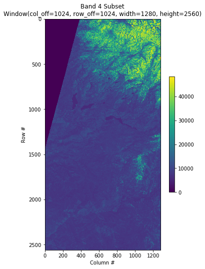
Let’s take a subset from high resolution image:
#https://rasterio.readthedocs.io/en/latest/topics/windowed-rw.html
#rasterio.windows.Window(col_off, row_off, width, height)
window = rasterio.windows.Window(1024, 1024, 1280, 2560)

with rasterio.open(fp) as src:
    subset = src.read(1, window=window)

plt.figure(figsize=(6,8.5))
plt.imshow(subset)
plt.colorbar(shrink=0.5)
plt.title(f'Band 4 Subset\n{window}')
plt.xlabel('Column #')
plt.ylabel('Row #')
<matplotlib.text.Text at 0x1b6fe014390>
These commands demonstrate the basics how to use COGs to retrieve data from the cloud.